Wave 2D (wave_2d)
Two-dimensional wave propagation on the periodic square. Disturbances spread as expanding rings, wrap around the box and interfere with themselves, so the target field is oscillatory at every scale the initial condition carried.
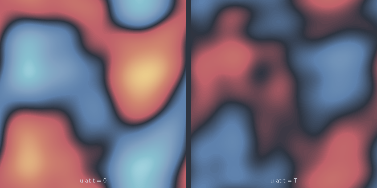
wave_2d): amplitude is conserved, the pattern is rearranged.Equation
with periodic boundary conditions and zero initial velocity.
Operator learning task
Parameters
| Parameter | Default | Range | Description |
|---|---|---|---|
wave_speed |
1.0 | (0.1, 10.0) | Propagation speed \(c\) |
time_end |
2.0 | (0.1, 20.0) | Final time \(T\) |
Usage
from pdeforge import generate_dataset

dataset = generate_dataset(
    model="wave_2d",
    n_samples=1000,
    resolution={"x": 64, "y": 64},
    params={"wave_speed": 1.0, "time_end": 2.0},
    seed=42,
)
Solver
Exact, with no time stepping at all. With zero initial velocity the solution in Fourier space is
applied in one shot at \(t = T\); a trajectory costs one transform per frame.
There is no dispersion error and no dissipation, whatever the horizon. That
exactness is what makes this model the reference for
heterogeneous_wave_2d, whose leapfrog scheme is
validated against this propagator in the constant-\(c\) limit.
Behaviour
Because energy is conserved and the domain is periodic, there is no long-time limit to relax into: the field keeps redistributing itself. That makes horizon length a genuine difficulty knob rather than a smoothing knob, since a longer run means more wraparound interference and a target less visibly related to its input.
Data shapes
Related
wave_1d: the one-dimensional version.heterogeneous_wave_2d: a spatially varying wave speed, with the medium as the operator's input.helmholtz_2d: the same physics in the frequency domain.