Lotka-Volterra 2D (lotka_volterra_2d)
The predator-prey oscillation with diffusion added. Without space, the classic system cycles forever on a closed orbit; add diffusion and the cycles at different points fall out of phase, so the oscillation turns into travelling population waves and patchy dynamics. The spatially uniform case reduces exactly to the textbook ordinary differential equations, and that reduction is used as the model's validation invariant.
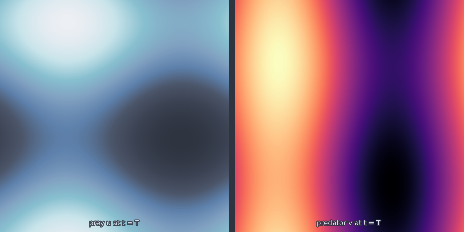
lotka_volterra_2d): the predator field trails the prey field it feeds on.Equation
on the periodic box.
Operator learning task
with components stacked on a leading axis, shape (2, ny, nx).
Parameters
| Parameter | Default | Range | Description |
|---|---|---|---|
a |
1.0 | (0.0, 10.0) | Prey growth rate |
b |
1.0 | (0.0, 10.0) | Predation rate |
c |
1.0 | (0.0, 10.0) | Predator death rate |
d |
1.0 | (0.0, 10.0) | Predator growth per prey |
Du |
0.01 | (0.0, 1.0) | Prey diffusivity |
Dv |
0.005 | (0.0, 1.0) | Predator diffusivity |
time_end |
5.0 | (0.1, 100.0) | Final time |
The coexistence fixed point sits at \((u, v) = (c/d,\; a/b)\), which is \((1, 1)\) at the defaults. Initial fields far from it produce large excursions and correspondingly large dynamic range in the target.
Usage
from pdeforge import generate_dataset

dataset = generate_dataset(
    model="lotka_volterra_2d",
    n_samples=500,
    resolution={"x": 128, "y": 128},
    params={"a": 1.0, "b": 1.0, "c": 1.0, "d": 1.0, "time_end": 5.0},
    seed=42,
)
Solver
The diagonal linear parts, meaning diffusion together with the linear growth and decay terms, ride in the exactly integrated operator; the \(uv\) coupling is stepped explicitly.
Behaviour
The unequal diffusivities matter: at the defaults the prey spreads twice as fast as the predator, so predator patches lag behind prey patches and the two fields are visibly offset in space. Setting \(D_u = D_v\) removes that offset and gives a far more predictable target.
Because the underlying kinetics is conservative rather than damped, there is no attractor to relax onto and long horizons keep producing new configurations.
Data shapes
Related
gray_scott_2d: reaction-diffusion where the kinetics select a stationary pattern.fitzhugh_nagumo_2d: two components with a threshold rather than a cycle.