Stokes 2D (stokes_2d)
Creeping flow, where inertia is absent and the response to a force is instantaneous and linear. That makes Stokes the natural first flow problem: the operator to be learned is genuinely a linear map, so any error is attributable to the representation rather than to nonlinearity. The incompressibility constraint is what gives it teeth, since it couples every point to every other.
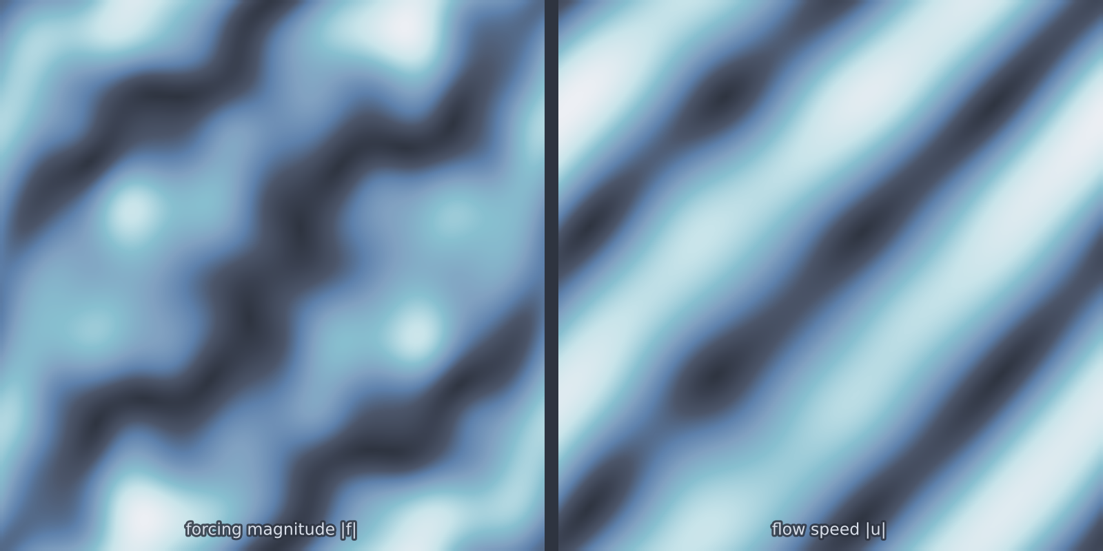
stokes_2d): the divergence-free constraint redistributes the response away from the forcing.Equation
on the periodic domain, with \(\mathbf{u} = (u, v)\) the velocity, \(p\) the pressure and \(\mathbf{f} = (f_x, f_y)\) a body force.
Operator learning task
Parameters
| Parameter | Default | Range | Description |
|---|---|---|---|
viscosity |
1.0 | (0.01, 100.0) | Dynamic viscosity \(\mu\); higher gives smoother velocity |
force_complexity |
5 | (1, 20) | Fourier modes in the random forcing |
force_complexity is the difficulty control, since it sets how multi-scale
the input measure is. At 1 the forcing is a single mode and the answer is a
single mode; at 20 the forcing spans a wide band and the viscous response
weights those bands very unevenly.
Usage
from pdeforge import generate_dataset

dataset = generate_dataset(
    model="stokes_2d",
    n_samples=1000,
    resolution={"x": 64, "y": 64},
    params={"viscosity": 1.0, "force_complexity": 5},
    seed=42,
)
Solver
Spectral, with the divergence-free constraint enforced exactly by Leray projection: the forcing is projected onto its solenoidal part in Fourier space, and what is removed is precisely the pressure gradient. No iteration and no saddle-point system, and the constraint holds to machine precision rather than to a tolerance.
This is the spectral Stokes
Despite sitting alongside the flow models that need FEniCSx, this one runs on the base installation. The domain is periodic, which is what makes the spectral solve possible.
Behaviour
Response amplitude scales as \(1/(\mu |\mathbf{k}|^2)\), so long-wavelength forcing produces far larger flow than short-wavelength forcing of the same amplitude. A dataset drawn from a broadband forcing measure therefore has outputs dominated by its lowest modes, and an operator can score well while ignoring most of the input spectrum. Reporting error band by band is more informative here than a single aggregate.
Data shapes
dataset.inputs.shape   # (n_samples, ny, nx, 2)   fx, fy
dataset.outputs.shape  # (n_samples, ny, nx, 3)   u, v, p
The component axis is trailing here. Several of the spectral multi-field models stack components on a leading axis instead, so check the shape rather than assuming a convention across the catalogue.
Related
cylinder_flow_2d: viscous flow with walls and inertia, solved by finite elements.ns_vorticity_2d: the same incompressibility with the nonlinear term restored.darcy_2d: the other steady spectral problem.