Navier-Stokes vorticity 2D (ns_vorticity_2d)
The most-cited operator-learning benchmark there is: two-dimensional incompressible Navier-Stokes in vorticity-streamfunction form, mapping the vorticity field at \(t = 0\) to the vorticity field at \(t = T\). Incompressibility enters through an elliptic solve for the streamfunction, which makes the velocity at any point depend on the vorticity everywhere, and that non-locality is the property the benchmark actually tests.
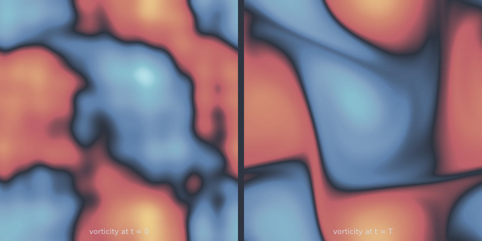
ns_vorticity_2d): the initial patches have merged and sheared into elongated sheets.Equation
on the periodic box.
Operator learning task
Parameters
| Parameter | Default | Range | Description |
|---|---|---|---|
viscosity |
1e-3 | (1e-5, 1.0) | Kinematic viscosity \(\nu\); lower is more turbulent |
time_horizon |
5.0 | (0.1, 100.0) | Final time \(T\) |
forcing |
"none" |
"none", "fno" |
"fno" adds the Li et al. (2020) steady forcing |
forcing_amplitude |
0.1 | (0.0, 10.0) | Forcing amplitude, used when forcing is on |
Usage
from pdeforge import generate_dataset

dataset = generate_dataset(
    model="ns_vorticity_2d",
    n_samples=1000,
    resolution={"x": 64, "y": 64},
    params={"viscosity": 1e-3, "time_horizon": 5.0},
    backend="jax",
    seed=42,
)

# the published forced setup, pinned
fno = generate_dataset(preset="fno_ns_vorticity_2d", n_samples=1000, seed=0)
The fno_ns_vorticity_2d preset sets \(\nu = 10^{-3}\), \(T = 50\) and the steady
forcing \(f = 0.1\,(\sin(2\pi(x+y)) + \cos(2\pi(x+y)))\) of the FNO paper.
The long-horizon preset is expensive
At \(T = 50\) and \(64^2\) on the NumPy backend, expect minutes per sample.
Pass backend="jax", shorten the horizon, or use n_jobs=-1.
Solver
ETDRK4 on the spectral seam: viscous diffusion exact, dealiased advection explicit. The streamfunction is recovered by dividing by \(|\mathbf{k}|^2\) in Fourier space, so the elliptic solve costs nothing beyond the transforms already being done.
Behaviour
Lower viscosity produces finer filaments, and filament width sets the resolution the dataset actually needs. Generating at \(64^2\) with \(\nu = 10^{-5}\) gives fields whose structure is at the grid scale, which means the data records the discretisation as much as the physics. When you lower \(\nu\), raise the resolution with it or expect the benchmark to measure aliasing.
Data shapes
Related
kolmogorov_flow_2d: the same solver with steady band forcing, giving a statistically steady turbulent state.burgers_2d: the same advection without incompressibility.cylinder_flow_2d_turbulent: turbulence with walls, solved by finite elements.