Stochastic heat 1D (stochastic_heat_1d)
The point at which the operator stops being a function. Add space-time noise to the heat equation and one initial condition no longer has one answer: it has a distribution. Every sample therefore carries several realisations of the same solve, which is the shape a distributional learning target actually needs and the reason PDEForge treats uncertainty as a property of the data rather than a post-processing step.
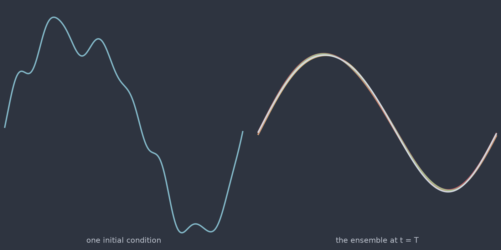
stochastic_heat_1d): the spread is the quantity being learned.Equation
where \(\dot{W}\) is space-time noise, expanded in Fourier modes as \(\dot{W}(x, t) = \sum_k \eta_k(t)\,e_k(x)\) with independent Brownian motions \(\eta_k\). Periodic boundary conditions.
Operator learning tasks
Two, and which one you want decides how you consume the output:
- Realisations. \(u_0 \mapsto \{u_T^{(1)}, u_T^{(2)}, \dots\}\), learning the conditional distribution directly.
- Moments. \(u_0 \mapsto (\mathbb{E}[u_T],\ \operatorname{Var}[u_T])\), learning the first two moments.
Parameters
| Parameter | Default | Range | Description |
|---|---|---|---|
diffusivity |
0.01 | (1e-6, 1.0) | Thermal diffusivity \(\alpha\) |
noise_intensity |
0.1 | (0.0, 1.0) | Noise amplitude \(\sigma\) |
n_realizations |
20 | (1, 200) | Realisations per initial condition |
time_end |
1.0 | (0.01, 10.0) | Final time; longer accumulates more noise |
n_realizations sets the quality of any moment estimate you take from the
data: the standard error of the sample mean falls as \(1/\sqrt{n}\), so 20
realisations give roughly 22% relative error on a per-point variance estimate
and 200 give about 7%.
Usage
from pdeforge import generate_dataset

dataset = generate_dataset(
    model="stochastic_heat_1d",
    n_samples=100,
    resolution={"x": 256},
    params={"diffusivity": 0.01, "noise_intensity": 0.1, "n_realizations": 50},
    seed=42,
)
dataset.outputs.shape   # (100, 50, 256): 50 realisations per initial condition
Solver
Exponential integrator for the exact viscous part with Euler-Maruyama
increments for the noise. Setting \(\sigma = 0\) recovers heat_1d
exactly, which is how the stochastic path is validated.
Behaviour
Diffusion and noise pull in opposite directions. Diffusion damps high wavenumbers; the noise injects them at every step. The stationary balance puts variance at mode \(k\) proportional to \(\sigma^2 / (2\alpha k^2)\), so the ensemble spread is dominated by long wavelengths while the fine structure stays close to the deterministic solution. An operator that predicts the mean well can still be badly wrong about the spread, which is the failure the calibration split exists to catch.
Data shapes
Related
heat_1d: the deterministic limit at \(\sigma = 0\).stochastic_heat_2d: the same model on the square.stochastic_burgers_1d: noise on top of nonlinear dynamics, where the spread is no longer Gaussian.- The calibration protocol, which is what these ensembles are generated for.