FitzHugh-Nagumo 2D (fitzhugh_nagumo_2d)
Excitable media on the square, where the extra dimension buys a phenomenon the line cannot host: a wavefront can break, and a broken front has free ends. Whether those ends curl into rotating spirals or retract and die is decided by the parameters, and the boundary between the two behaviours is sharp.
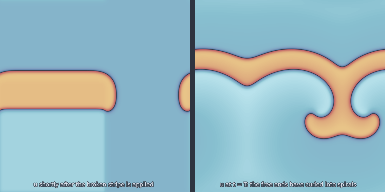
fitzhugh_nagumo_2d): the excitable recipe at beta = 0.5, on one colour scale.Equation
with periodic boundary conditions.
Operator learning task
As in one dimension, the stored input is the activator field alone; both
components come back. To vary the inhibitor as well, build the model directly
and pass ic_v to solve, as in the spiral recipe below.
Parameters
| Parameter | Default | Range | Description |
|---|---|---|---|
epsilon |
0.08 | (0.01, 0.5) | Timescale separation; smaller gives sharper waves and spirals |
diffusivity_u |
1.0 | (0.01, 10.0) | Activator diffusion, setting wave speed and pattern scale |
time_end |
50.0 | (1.0, 200.0) | Final time |
Excitability regimes
These were established numerically, and the test that pins them is
tests/test_new_models.py::test_fhn_broken_front_regimes.
At the default \(\beta = 0.7\) the medium is sub-excitable: plane fronts propagate, but a broken wavefront retracts from its free ends and dies, so no spiral can form from a wave break. Around \(\beta = 0.5\) with \(\epsilon \approx 0.02\) the medium is fully excitable: broken fronts curl at the tips, collide and re-seed indefinitely. Excitation seeds must span roughly 8 units of \(\sqrt{D_u}\) for a pulse to launch at all.
The site's motion loop uses the excitable recipe; the code is
motion_fhn_spiral in scripts/make_gallery.py.
Usage
from pdeforge import generate_dataset

dataset = generate_dataset(
    model="fitzhugh_nagumo_2d",
    n_samples=200,
    resolution={"x": 128, "y": 128},
    params={"epsilon": 0.08, "time_end": 50.0},
    seed=42,
)
The default measure mostly records decay
Two things work against excitation in the call above. The default
\(\beta = 0.7\) is sub-excitable, and when solve is given no ic_v it puts
every point on the \(v\)-nullcline, including the stimulus, so there is no
recovery lag for a pulse to exploit. A dataset generated this way is largely
a dataset of decaying bumps. Set the medium to its rest state and stimulate
from there, as below.
For the spiral regime, build the model directly so the initial condition can carry a deliberate wave break:
from pdeforge import get_model
import numpy as np

beta, gamma = 0.5, 0.8
u_rest = -0.76                       # most negative root of gamma u^3 + (1-gamma) u + beta
m = get_model("fitzhugh_nagumo_2d")(
    resolution={"x": 256, "y": 256},
    domain={"x": (0.0, 120.0), "y": (0.0, 120.0)},
    epsilon=0.02, beta=beta, time_end=400.0,
)
X, Y = np.meshgrid(m.grids["x"], m.grids["y"])
v_rest = (u_rest + beta) / gamma
u0 = np.full_like(X, u_rest)
v0 = np.full_like(X, v_rest)
u0[(np.abs(Y - 60.0) < 8.0) & (X < 66.0)] = 1.0    # a broken stripe
v0[(Y < 52.0) & (X < 66.0)] = v_rest + 0.45        # refractory block: the tips curl
traj = m.solve(u0, ic_v=v0, return_full=True)      # (n_t, ny, nx, 2)
Passing ic_v explicitly is what makes this work: it holds the medium at rest
so the stimulus sits above threshold rather than on the nullcline. The figure
at the top of this page is traj[2] against traj[-1], and
scripts/make_model_figures.py regenerates it.
Data shapes
dataset.inputs.shape   # (n_samples, ny, nx)      u0
dataset.outputs.shape  # (n_samples, ny, nx, 2)   u_T, v_T on a trailing axis
Note that the component axis is trailing here, unlike the leading axis used by
gray_scott_2d and burgers_2d.
Related
fitzhugh_nagumo_1d: the same system where fronts cannot break.gray_scott_2d: stationary patterns rather than travelling waves.allen_cahn_2d: the cubic nonlinearity without an inhibitor.