Transonic Airfoil Euler (airfoil_euler_2d)
Steady compressible Euler around a parameterised NACA 4-digit airfoil, marched to steady state on a body-fitted C-grid. At the transonic condition the flow accelerates past Mach 1 over the upper surface and closes with a shock, which is the feature that makes this a genuinely different learning problem from every smooth model in the catalogue, and one a Fourier method would ring across.
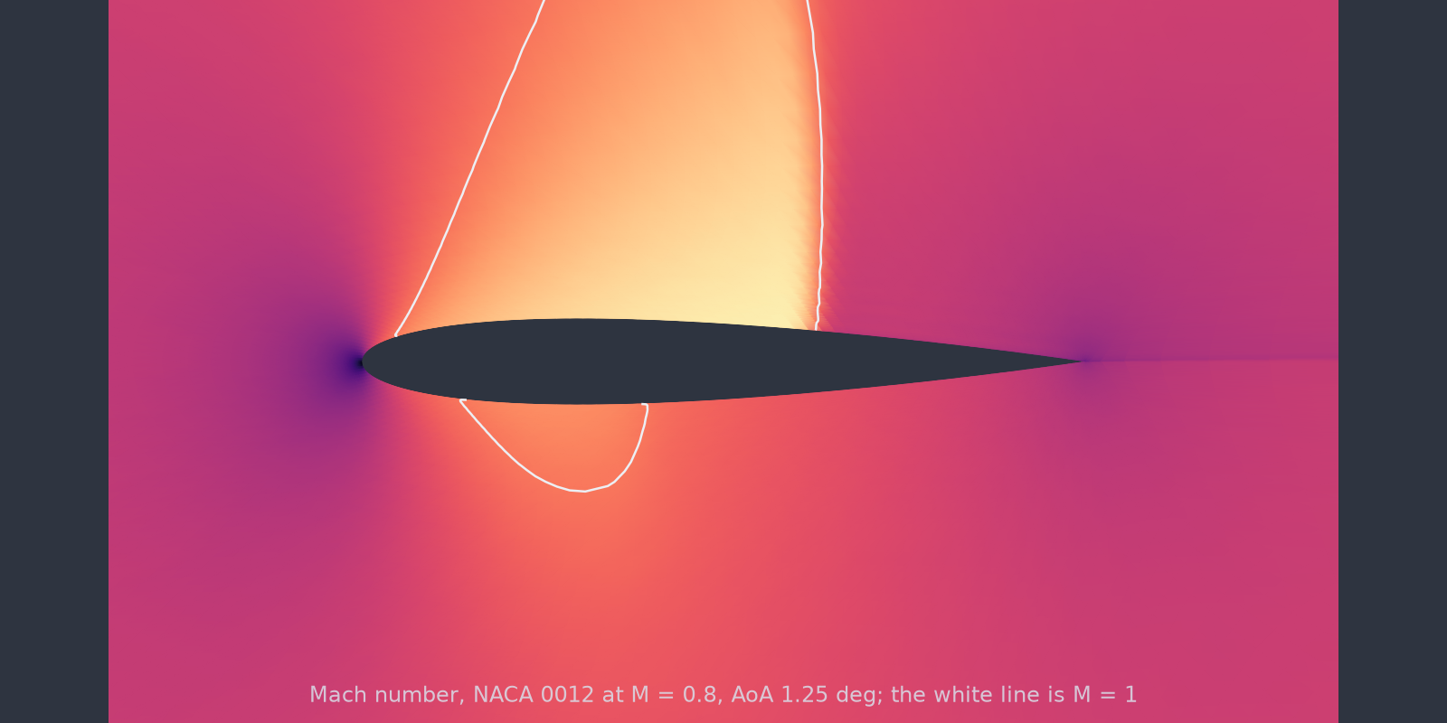
airfoil_euler_2d): the white line is the sonic boundary, and the shock closes the supersonic pocket.Equations
with cell-centred finite volumes, HLLC fluxes, MUSCL/minmod reconstruction and a local time step.
Operator learning task
Every sample draws its own airfoil, meaning thickness, camber and camber position, and its own flow condition, meaning freestream Mach and angle of attack. The mesh is rebuilt around it and the solution returned on that mesh, so the task is the Geo-FNO one, a deformed mesh in and the field on it out, rather than a fixed Cartesian grid:
Parameters
| Parameter | Default | Description |
|---|---|---|
mach_range |
(0.70, 0.82) | Freestream Mach draw range |
aoa_range |
(-1.5, 3.0) | Angle-of-attack draw range, in degrees |
thickness_range |
(0.08, 0.15) | NACA thickness draw range |
camber_range |
(0.0, 0.04) | Maximum camber draw range |
camber_pos_range |
(0.3, 0.5) | Camber position draw range |
cfl |
0.7 | Local time-step CFL number |
max_iterations |
12000 | Iteration cap for the steady march |
residual_tol |
1e-5 | Convergence tolerance |
Usage
No extra install: this is pure NumPy.
from pdeforge import generate_dataset

dataset = generate_dataset(
    model="airfoil_euler_2d",
    n_samples=200,
    resolution={"xi": 256, "eta": 64},   # C-grid cell counts
    params={"mach_range": (0.70, 0.82), "aoa_range": (-1.5, 3.0)},
    seed=0,
)
dataset.inputs.shape           # (200, 256, 64, 2)  the deformed mesh
dataset.outputs.shape          # (200, 256, 64, 4)  rho, u, v, p
dataset.metadata["Cl"]                   # per-sample lift coefficient
dataset.metadata["Cd"]                   # per-sample drag coefficient
dataset.metadata["mach_max"]             # peak Mach reached in each sample
dataset.metadata["transonic_fraction"]   # share of samples with a shock
dataset.metadata["param_samples"]        # the drawn geometry and flow condition
xi wraps the airfoil and both wake cuts, and eta runs from the wall to the
far field. xi is rounded to even so the surface point count stays odd and the
sharp trailing edge lands on a node; the Kutta condition then emerges from the
geometry and the wake cut rather than being enforced.
Validation
Four checks, in increasing strength:
| Check | Result |
|---|---|
| Freestream preservation away from the wall, and across the wake cut | residual \(\sim 10^{-13}\) (geometric conservation law; the cut is transparent) |
| NACA 0012, \(M=0.5\), \(\alpha=0\): d'Alembert says \(C_l = C_d = 0\) | \(C_l = 0.002\), \(C_d = 0.0035\); the drag is purely scheme dissipation, and falls 8x from first to second order |
| Stagnation \(C_p\) against the exact compressible value 1.064 | 1.017 |
| NACA 0012, \(M=0.8\), \(\alpha=1.25°\) against the published inviscid benchmark | shock within 1% of station; forces about 10% out (see below) |
The transonic case is the one that matters and the one to read carefully:
| Grid | \(C_l\) | \(C_d\) | shock \(x/c\) | \(M_{\max}\) |
|---|---|---|---|---|
| \(161 \times 65\) | 0.318 | 0.0259 | 0.626 | 1.357 |
| \(241 \times 81\) | 0.321 | 0.0240 | 0.623 | 1.364 |
| published | 0.352 | 0.0224 | 0.62 |
The shock lands within 1% of the published station and stays there under refinement, and the supersonic pocket peaks at \(M \approx 1.36\): the flow structure is right, which is what a field-predicting dataset is for. The force coefficients are about 10% low in lift and 7 to 15% high in drag, both moving the right way with refinement, so this is discretisation rather than a modelling error, and neither run reached its convergence tolerance within the iteration cap.
So treat the fields as the product and the forces as indicative. Closing
the last few percent on integrated forces is a tuning exercise, covering
wall-pressure extrapolation, deeper convergence and finer meshes, that this
model does not claim to have done. This comparison runs under PDEFORGE_SLOW=1
and takes minutes per grid.
This model is expensive
A steady transonic solve is thousands of explicit iterations. At
\(256 \times 64\) expect minutes per sample, so pass n_jobs=-1 for anything
beyond a handful: process-parallel generation is supported and bit-identical
to sequential.
Not a recreation of anything
This is airfoil data with knobs at a shock-carrying condition. It is not a
byte-level recreation of the Geo-FNO airfoil dataset, whose mesh, solver and
sampling are their own, and it is emphatically not RANS: for the
viscous, turbulence-closed regime PDEForge
reads AirfRANS rather than rebuilding it. For
incompressible airfoil flow with a real viscous wake, see
naca_flow_2d.
Related
naca_flow_2d: incompressible laminar flow past the same airfoil family, solved by finite elements.cylinder_flow_2d_parameterized: the other geometry-varying model.burgers_1d: the catalogue's other shock-forming model, in one dimension and with viscosity holding the front.