KdV 1D (kdv_1d)
One model, one solver, several regimes. The Korteweg-de Vries equation is the canonical dispersive PDE: \(\text{sech}^2\) solitary waves travel at a speed set by their own amplitude and pass through each other unchanged. The published KdV setups in the operator-learning literature differ only in their coefficients, box size and input measure, so they ship here as presets on one model instead of as separate models.
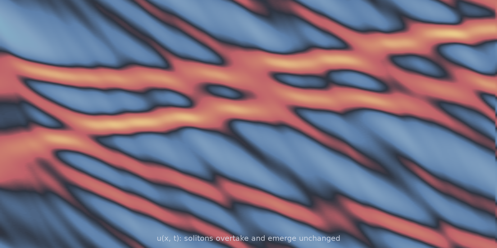
kdv_1d): solitons of different amplitudes cross repeatedly and re-emerge with their shapes intact.Equation
on a periodic box. Defaults are the textbook normalisation: \(\mu = 6\), \(\delta^2 = 1\) on \([0, 20]\), with a soliton input measure.
Operator learning task
or the whole trajectory with outputs="trajectory".
Parameters
| Parameter | Default | Range | Description |
|---|---|---|---|
time_end |
1.0 | (0.01, 200.0) | Final time \(T\) |
advection |
6.0 | (0.1, 20.0) | Coefficient \(\mu\) on \(u u_x\); textbook KdV is 6 |
dispersion |
1.0 | (1e-6, 10.0) | Coefficient \(\delta^2\) on \(u_{xxx}\) |
dealias |
True |
2/3 rule on the nonlinear term | |
scale_jitter |
0.0 | Per-trajectory randomisation of box and horizon |
Presets
| Preset | Regime |
|---|---|
| (model default) | Solitons: \(\mu=6\), \(\delta^2=1\), \(L=20\), elastic collisions |
kdv_dsw_1d |
Undular bore, \(\delta^2 = 8\times10^{-6}\): un-resolvable bias set |
kdv_dsw_epistemic_1d |
Undular bore, \(\delta^2 = 4\times10^{-5}\): near-resolvable |
mp_pde_kdv_1d |
Brandstetter et al. benchmark, \(\mu=\delta^2=1\), \(L=128\) |
mp_pde_kdv_easy_1d |
The same at \(T = 50\) |
Usage
from pdeforge import generate_dataset

# textbook solitons
dataset = generate_dataset(
    model="kdv_1d",
    n_samples=1000,
    resolution={"x": 256},
    params={"advection": 6.0, "dispersion": 1.0, "time_end": 1.0},
    seed=42,
)

# a published regime, pinned
bore = generate_dataset(preset="kdv_dsw_1d", n_samples=1000, seed=0)
Solver
The stiff dispersion term has symbol \(i\,\delta^2 k^3\), which is integrated exactly by ETDRK4: the stiffness that cripples explicit schemes never appears in the time step, and only \(\mu\,u u_x\) is stepped. That is what makes the small-\(\delta^2\) bore regimes affordable at all.
Dispersive shock waves (kdv_dsw_1d, kdv_dsw_epistemic_1d)
A localised smooth depression (the depression_box input measure) does not
steepen into a thin front. Under KdV it dissolves into a dispersive shock
wave, an undular bore: sustained high-wavenumber oscillations filling a
large, contiguous region. Where a Burgers shock mis-samples only a
\(\sqrt{\nu}\)-thin front, the bore is hard for a band-limited operator
everywhere it lives, which makes it a stringent operator and UQ benchmark.
The two bore presets are a matched pair. At \(n_x = 512\) the vigorous bore (\(\delta^2 = 8\times10^{-6}\)) shows about 155 oscillations but is not grid converged: it has about 429 at \(n_x = 2048\), so its hardness is a bias floor no amount of data removes. The longer-wavelength bore (\(4\times10^{-5}\)) shows about 83 oscillations and is already converged at \(n_x = 512\), so its hardness is epistemic, meaning data-limited. That contrast is what makes them useful together for method comparison.
Spectral centroid will mislead you here
With dealiasing on, the 2/3 mask truncates the \(8\times10^{-6}\) bore, so its spectral centroid reads lower (3.8) than the resolvable bore's (10.3) despite having the shorter wavelength. Count oscillations rather than centroid: the truncation is the phenomenon, and not an artefact to average over.
The neural-emulator benchmark regime (mp_pde_kdv_1d)
Brandstetter et al. (Message Passing Neural PDE Solvers, arXiv:2202.03376; Lie Point Symmetry Data Augmentation, arXiv:2202.07643) use \(\mu = \delta^2 = 1\) on a long \(L = 128\) box. That whole setup ships as a preset:
dataset = generate_dataset(preset="mp_pde_kdv_1d", n_samples=512, seed=0)
# -> inputs (512, 256), outputs (512, 140, 256) trajectories
The preset pins the four things that make that regime what it is:
| Setting | Value | Why it matters |
|---|---|---|
advection, dispersion |
1.0, 1.0 |
Not the textbook \(\mu = 6\); a different soliton amplitude-speed law |
ic_generator="sine_series" |
10 waves, \(l \in \{1, 2\}\) | Long-wave random sine series (see below) |
scale_jitter |
0.1 |
Each trajectory draws its own \(L\) and \(T\) within \(\pm 10\%\) |
_n_frames_kept |
140 of 250 |
Trajectories start at \(t \approx 0.44\,T\), from a developed soliton gas |
The input measure. sine_series (TruncatedSineGenerator) draws
with \(A_j \sim U(-0.5, 0.5)\), \(\phi_j \sim U(0, 2\pi)\), and integer \(l_j\) from the half-open range \([l_\min, l_\max)\). The canonical \((1, 3)\) therefore excites modes 1 and 2, with mode 3 excluded by the half-open convention; closing the interval would silently widen the measure. The field is exactly zero-mean on a uniform periodic grid, which KdV then conserves.
Scale jitter. KdV's scaling symmetry
\((u, x, t) \mapsto (\lambda^2 u, x/\lambda, t/\lambda^3)\) is what makes a
randomised box worth having rather than a relabelling. Because this measure is
a function of \(x/L\), jitter leaves the initial conditions untouched and
perturbs only the dynamics. Note that the dataset's stored grid stays
nominal: per-sample \(dx\) and \(dt\) differ from it by up to the jitter
fraction, so the genuinely shared coordinate is \(x/L\). Jitter requires
backend="numpy".
Dealiasing. The preset sets dealias=False to match the reference
generator's psdiff right-hand side. This is not fidelity theatre: at
\(n_x = 256\) the 2/3 mask also removes genuine spectral content once KdV has
broadened the spectrum. Measured against a converged \(n_x = 1024\) reference at
\(T = 100\), un-dealiased ETDRK4 sits at \(8 \times 10^{-7}\) relative \(L^2\),
dealiased at \(1 \times 10^{-4}\), and the reference generator's own
Radau plus psdiff scheme at \(2.9 \times 10^{-4}\). _dt = 5e-3 is converged
there.
Data shapes
dataset.inputs.shape   # (n_samples, nx)
dataset.outputs.shape  # (n_samples, nx)  or (n_samples, n_t, nx) for trajectories
Related
burgers_1d: the same nonlinearity with diffusion instead of dispersion, and a thin shock instead of a bore.schrodinger_1d: the other dispersive 1D model.ks_1d: the chaotic member of the family.