Kuramoto-Sivashinsky 1D (ks_1d)
The canonical chaotic PDE. Energy enters at long wavelengths through the
destabilising \(-u_{xx}\) term and leaves at short ones through hyperdiffusion,
with the nonlinearity ferrying it between the two. Above a domain size of
roughly 20 the result is spatiotemporal chaos on a finite-dimensional
attractor, which makes ks_1d the model for the question of whether an
operator has learned dynamics or learned to interpolate.
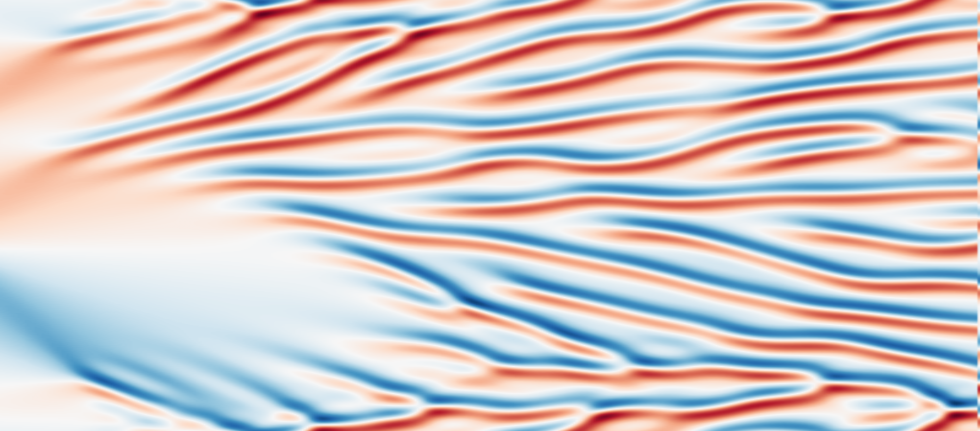
ks_1d): chaos develops once the domain size exceeds about 20.Equation
on a periodic domain, default size \(32\pi\): the classic setup of Kassam and Trefethen (2005).
Operator learning task
Parameters
| Parameter | Default | Range | Description |
|---|---|---|---|
time_horizon |
50.0 | (1.0, 500.0) | Final time \(T\); chaos develops over \(t \gtrsim 50\) |
Domain size is the other control, set through domain= rather than params=.
It is the physically meaningful bifurcation parameter here, since the number
of linearly unstable modes grows with \(L\).
Usage
from pdeforge import generate_dataset

dataset = generate_dataset(
    model="ks_1d",
    n_samples=1000,
    resolution={"x": 256},
    params={"time_horizon": 50.0},
    seed=42,
)

# a longer, more strongly chaotic run
long_run = generate_dataset(
    model="ks_1d",
    n_samples=100,
    resolution={"x": 512},
    params={"time_horizon": 150.0, "_n_time_steps": 400},
    outputs="trajectory",
    seed=3,
)
Solver
The linear symbol \(k^2 - k^4\) is integrated exactly by ETDRK4, and only the dealiased advective nonlinearity is stepped explicitly. Treating \(-u_{xxxx}\) explicitly would force a time step scaling as \(\Delta x^4\), so the exponential integrator is what makes long horizons practical.
Behaviour
Chaos sets a hard ceiling on what any operator can do at long horizon. Trajectories with nearby initial conditions separate exponentially, so beyond a few Lyapunov times the pointwise map is not learnable in principle, whatever the architecture. Two consequences follow for benchmark design. Short horizons measure the operator; long horizons measure the attractor, and should be scored on statistics rather than pointwise error. And a model that looks excellent at \(T = 5\) and collapses at \(T = 100\) is behaving correctly, so the horizon has to be reported alongside the number.
Data shapes
Related
burgers_1d: the same nonlinearity, without the energy injection that makes this one chaotic.kolmogorov_flow_2d: forced chaos in two dimensions, with a statistically steady state.kdv_1d: dispersive rather than dissipative.