Canonical FNO Darcy (darcy_fno_2d)
The Darcy benchmark of Li et al. (2021), regenerable. This is a transcription
of the published MATLAB generator (GRF.m + solve_gwf.m), not an
approximation of it: solving the distributed 421 x 421 coefficients returns
the distributed solutions with 99.1% of the 177,241 float32 values
identical and none more than 2 ulp out. That residue is MATLAB's sparse LU
against SciPy's, and nothing else.
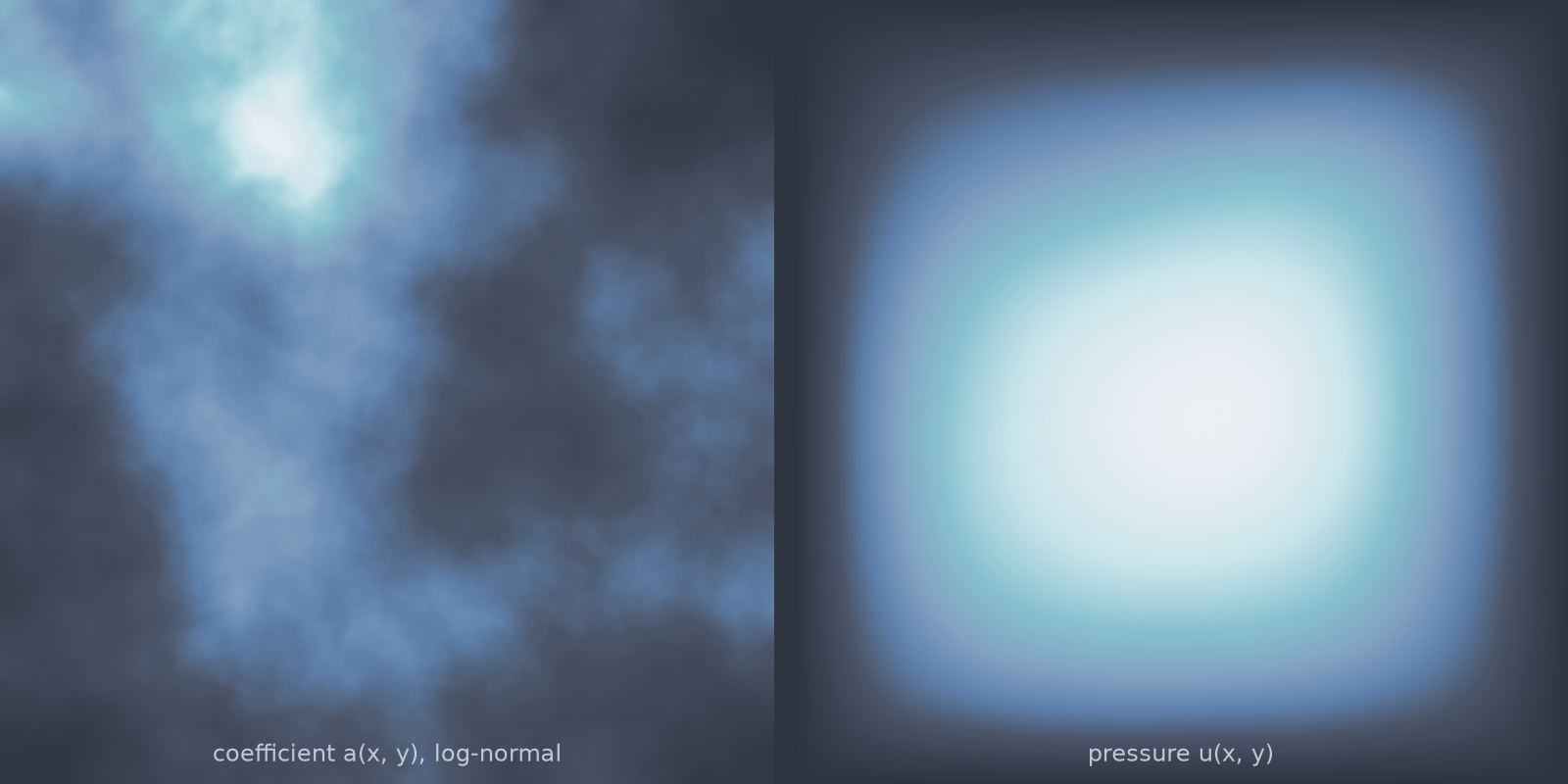
darcy_fno_2d).Equation
Operator learning task: \(a(x,y) \mapsto u(x,y)\).
The input measure
Coefficients come from the canonical Gaussian measure
with zero-Neumann Laplacian, sampled by Karhunen-Loeve expansion in the cosine (DCT) basis. Two pushforwards make it elliptic:
coeff="lognormal": \(a = e^{\psi}\), the Darcy421 family.coeff="piececonst": \(a = \kappa_+\) where \(\psi \ge\)threshold, else \(\kappa_-\); the distributed two-phase files use 12 and 3.
The field scale is not a free parameter: the \(\tau^{\alpha-1}\)
normalisation fixes it, giving \(\sigma = 0.292083\) at the canonical
\(\alpha = 2, \tau = 3\). Pass a number for sigma only when the contrast
is the knob you want; leave it None and \(\alpha\) and \(\tau\) stay
honest knobs.
The grid convention, which decides everything downstream
The published generator does something no one would guess from the data. It solves on the node grid, \(K\) points at \(i/(K-1)\) with zero Dirichlet at the boundary nodes, but takes its input and returns its output on the cell-centre grid, \(K\) points at \((2i+1)/(2K)\), moving between the two with a not-a-knot cubic spline.
So the distributed arrays are samples of a node-grid solution at cell centres, half a cell inside the wall. That is why their boundary values are small but not zero, and why reading them as a plain node-grid solve leaves a 0.49% discrepancy no amount of solver polish removes.
grid |
Fields sampled at | Boundary | Use for |
|---|---|---|---|
"canonical" (default) |
cell centres, \((2i+1)/(2K)\) | small, nonzero | reproducing the published arrays |
"node" |
nodes, \(i/(K-1)\) | exactly zero | new data (no resampling error) |
Parameters
| Parameter | Default | Description |
|---|---|---|
coeff |
"lognormal" |
lognormal or piececonst |
grid |
"canonical" |
canonical or node (see above) |
alpha |
2.0 | GRF spectral decay; higher is smoother |
tau |
3.0 | GRF inverse correlation length |
sigma |
None |
None = canonical \(\tau^{\alpha-1}\); a number overrides |
kappa_plus / kappa_minus |
12.0 / 3.0 | two-phase permeabilities |
threshold |
0.0 | level-set threshold, in units of \(\sigma\) |
forcing |
1.0 | constant source \(f\) |
Usage
from pdeforge import generate_dataset

# the canon, at a resolution no distributed file offers
dataset = generate_dataset(
    preset="fno_darcy_2d", n_samples=1000,
    resolution={"x": 601, "y": 601}, seed=0,
)

# the same physics without the original's resampling
clean = generate_dataset(
    preset="fno_darcy_clean_2d", n_samples=1000,
    resolution={"x": 256, "y": 256}, seed=0,
)

# a rougher measure than the canon ever shipped
rough = generate_dataset(
    model="darcy_fno_2d", n_samples=1000, resolution={"x": 256, "y": 256},
    params={"alpha": 1.5, "tau": 7.0}, seed=0,
)
A 421 x 421 sample costs about 1.1 s (sparse LU), so the full 5000-sample canonical set is a couple of CPU-hours.
Reading the distributed files
The files are torch.save archives; pdeforge.read_torch_pt reads them as
memory-mapped numpy arrays without PyTorch, so inspecting 7 GB of
benchmark data does not pull in a deep-learning framework. The grid returned
is the cell-centre one the data is actually sampled on.
Note that the distributed low-resolution files (211, 141, 106, 85) are
strided views of the 421 master grid, not independent runs. resolution=
in the loader takes those strides and refuses anything else. Regenerating at
a resolution instead gives a genuinely independent discretisation of the same
measure, which is a different and usually more useful thing.
Solver
Five-point flux-form finite differences with arithmetic face averaging (the
original's choice; _face_average="harmonic" is available), assembled sparse
and solved by direct LU. In grid="node" the discrete operator residual is
machine precision, and against the classical series solution for \(a=1\) the
solve converges at the expected second order.
Related
darcy_fno_3d: the same measure and solver on the unit cube, where no frozen dataset exists.porous_darcy_fem: Darcy flow through Cahn-Hilliard microstructures (FEM).darcy_2d: the periodic spectral Darcy, a different problem.