Burgers 2D (burgers_2d)
The vector generalisation of Burgers: a two-component velocity advecting
itself, with no pressure and no incompressibility constraint. That omission is
the point. Sharp fronts form and diffuse in two dimensions without the elliptic
coupling that makes Navier-Stokes global, so this sits between
burgers_1d and ns_vorticity_2d as a
genuinely two-dimensional problem that stays local.
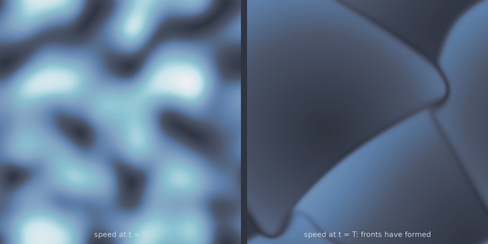
burgers_2d): the smooth initial field has collapsed onto fronts.Equation
on the periodic box.
Operator learning task
with the components stacked on a leading axis, shape (2, ny, nx).
Parameters
| Parameter | Default | Range | Description |
|---|---|---|---|
viscosity |
0.01 | (1e-5, 1.0) | Viscosity \(\nu\); lower gives sharper fronts |
time_horizon |
1.0 | (0.05, 10.0) | Final time \(T\) |
Usage
from pdeforge import generate_dataset

dataset = generate_dataset(
    model="burgers_2d",
    n_samples=1000,
    resolution={"x": 128, "y": 128},
    params={"viscosity": 0.01, "time_horizon": 1.0},
    seed=42,
)
Solver
ETDRK4 on the spectral seam: viscous diffusion exact, dealiased self-advection explicit for both components. Same machinery as the one-dimensional model, applied twice.
Behaviour
Two-dimensional fronts are curves rather than points, so the region a low-viscosity solution puts its error in scales as \(\sqrt{\nu}\) in width but spans the domain in length. The practical effect is that the difficult set is a much larger share of the field than in one dimension at the same viscosity, and resolution requirements bite sooner.
Data shapes
Related
burgers_1d: the scalar version, with published presets.ns_vorticity_2d: add incompressibility and the dynamics become global.shallow_water_2d: the other multi-component hyperbolic system.