Allen-Cahn 3D (allen_cahn_3d)
Non-conserved phase separation in three dimensions. Domains of the \(\pm 1\)
wells coarsen by mean-curvature flow of their interfaces, which are now
surfaces. The physics is the same as in allen_cahn_2d;
what changes is that the interface is a two-dimensional object embedded in a
volume, so the fraction of the grid carrying the useful signal falls again.
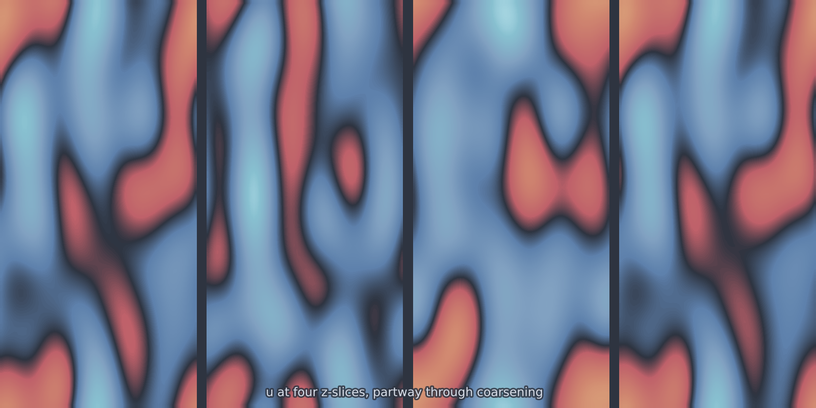
allen_cahn_3d).Equation
on the periodic cube.
Operator learning task
Parameters
| Parameter | Default | Range | Description |
|---|---|---|---|
epsilon |
0.01 | (0.001, 0.5) | Interface width |
time_end |
5.0 | (0.1, 100.0) | Final time |
Usage
from pdeforge import generate_dataset

dataset = generate_dataset(
    model="allen_cahn_3d",
    n_samples=200,
    resolution={"x": 64, "y": 64, "z": 64},
    params={"epsilon": 0.01, "time_end": 5.0},
    seed=42,
    to="ac3d.h5",     # chunked to disk
)
Solver
ETDRK4 on the dimension-agnostic seam, exactly as in one and two dimensions: the linear operator including the linear part of the reaction is integrated exactly, the cubic term explicitly.
Mind the memory
A \(64^3\) float64 field is 2 MB, so inputs and outputs together are 4 MB per
sample. Pass to= for anything past a few hundred samples and let the
generator stream chunks to disk.
Behaviour
Interfaces occupy a shrinking share of the volume as \(\varepsilon\) falls: at \(\varepsilon = 0.01\) on a \(64^3\) grid, the transition region is a few cells thick around surfaces that themselves cover a small part of the box. Most voxels sit at \(\pm 1\) and carry no information, which flatters any error metric averaged over the volume. Score on the interface region if the interface is what you care about.
Data shapes
Related
allen_cahn_1d,allen_cahn_2d: the lower-dimensional versions.cahn_hilliard: runs in 3D from the same code path, with conserved dynamics.heat_3d: the linear volumetric baseline.