Allen-Cahn 1D (allen_cahn_1d)
Phase separation with non-conserved dynamics. The double-well potential \(f(u) = (1 - u^2)^2/4\) has minima at \(u = \pm 1\), so an arbitrary initial field is driven towards a piecewise-constant state joined by interfaces of width \(O(\sqrt{\varepsilon})\). What an operator has to learn here is where the interfaces end up, and that is a discrete outcome hiding inside a smooth map: two nearby initial conditions can put an interface in different places, or leave one out entirely.
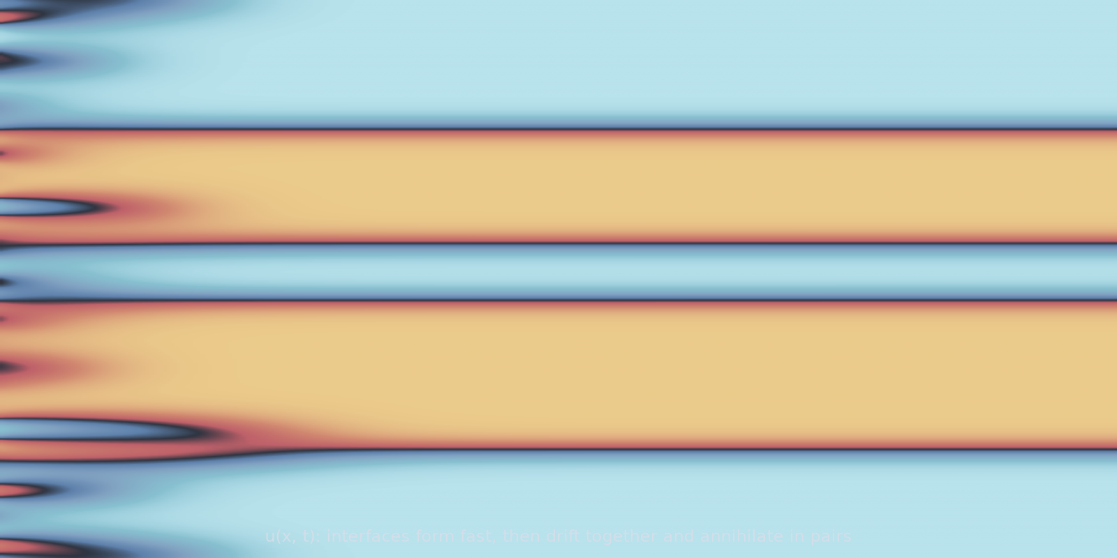
allen_cahn_1d): interfaces form quickly, then drift together and annihilate in pairs.Equation
with periodic boundary conditions.
Operator learning task
Parameters
| Parameter | Default | Range | Description |
|---|---|---|---|
epsilon |
0.01 | (0.001, 0.5) | Interface width; smaller gives sharper phase boundaries |
time_end |
10.0 | (0.1, 100.0) | Final time; longer gives more complete separation |
Usage
from pdeforge import generate_dataset

dataset = generate_dataset(
    model="allen_cahn_1d",
    n_samples=1000,
    resolution={"x": 256},
    params={"epsilon": 0.01, "time_end": 10.0},
    seed=42,
)
Solver
ETDRK4 on the spectral seam, with the linear part of the reaction folded into the exactly integrated operator alongside diffusion. Only the cubic term is stepped explicitly.
Behaviour
Two stages, on very different timescales. Interfaces form fast, in a time set
by the linear growth rate of the unstable \(u = 0\) state. After that the
dynamics are slow: interfaces move by curvature, drift together and annihilate
in pairs, and the number of domains falls logarithmically. Choosing
time_end therefore chooses which of those two problems the dataset poses.
Small \(\varepsilon\) needs resolution to match. The interface is \(O(\sqrt{\varepsilon})\) wide, so at \(\varepsilon = 0.001\) on 256 points the transition spans only a few cells, and the sampled data starts to depend on where the grid happens to fall.
Data shapes
Related
allen_cahn_2d,allen_cahn_3d: the same equation with curvature-driven coarsening in higher dimensions.cahn_hilliard: the conserved counterpart, where the mean composition is preserved exactly.stochastic_allen_cahn_2d: noise-driven selection between the wells, which is where the outcome becomes genuinely random.