Elasticity 2D (elasticity_2d)
The elasticity analogue of the Darcy coefficient-to-solution map: hand the operator a heterogeneous stiffness field and ask for the displacement and stress it produces under a fixed load. Stiff inclusions concentrate stress at their boundaries, so the von Mises output has sharp features in places the input only marks by a change of value.
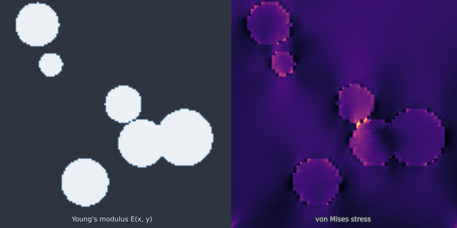
elasticity_2d): stress concentrates around the stiff inclusions.Equation
Plane-strain linear elasticity on the unit square,
with the Lamé fields derived from a heterogeneous Young's modulus \(E(\mathbf{x})\): a matrix phase seeded with random circular inclusions of contrasting stiffness. The bottom edge is clamped, a uniform traction acts on the top edge, and the sides are free.
Operator learning task
Parameters
| Parameter | Default | Range | Description |
|---|---|---|---|
e_matrix |
1.0 | (0.01, 100.0) | Young's modulus of the matrix phase |
e_inclusion |
10.0 | (0.01, 1000.0) | Modulus of the inclusions; above 1 stiff, below 1 soft |
poisson |
0.3 | (0.05, 0.45) | Poisson ratio, uniform |
traction_x |
0.0 | (-10.0, 10.0) | Traction \(x\)-component on the top edge |
traction_y |
-1.0 | (-10.0, 10.0) | Traction \(y\)-component; negative compresses towards the clamp |
n_inclusions |
6 | (0, 40) | Number of random circular inclusions |
The traction components are physical parameters rather than fixed geometry, so the UQ layer can draw them per sample alongside the random inclusions.
Usage
from pdeforge import generate_dataset

dataset = generate_dataset(
    model="elasticity_2d",
    n_samples=100,
    resolution={"x": 64, "y": 64},
    params={"e_inclusion": 10.0, "traction_y": -1.0, "n_inclusions": 6},
    seed=42,
)
This model needs FEniCSx. See FEniCSx setup.
Validation
Clapeyron's theorem. For the discrete Galerkin solution the strain energy equals half the external work exactly, by taking the test function to be the solution itself, so the energy balance checks assembly and solver together at solver precision rather than at discretisation accuracy.
Behaviour
Stiffness contrast is the difficulty knob. At e_inclusion far from
e_matrix in either direction, the stress field develops steep gradients at
the inclusion boundaries, and those boundaries are circles that the mesh
resolves rather than the grid. Soft inclusions (\(E < 1\)) behave differently
from stiff ones: they shed load rather than attracting it, so the stress
concentrates in the matrix between them.
Data shapes
dataset.inputs.shape   # (n_samples, nx, ny)      E
dataset.outputs.shape  # (n_samples, nx, ny, 3)   u, v, von Mises
The FEniCSx models store space as (nx, ny) with the component axis trailing,
which is transposed relative to the spectral models' (ny, nx). Transpose
before plotting.
Related
darcy_fno_2d: the same coefficient-to-solution shape, for a scalar elliptic problem.porous_darcy_fem: the other FEniCSx model built on a generated microstructure.