Heat 2D (heat_2d)
Isotropic diffusion on the square. The map is the same low-pass filter as in one dimension, now with the decay rate set by \(|\mathbf{k}|^2 = k_x^2 + k_y^2\), which means the corner modes of the spectrum die far faster than the axis modes. Structures shrink into blobs, and the blobs merge.
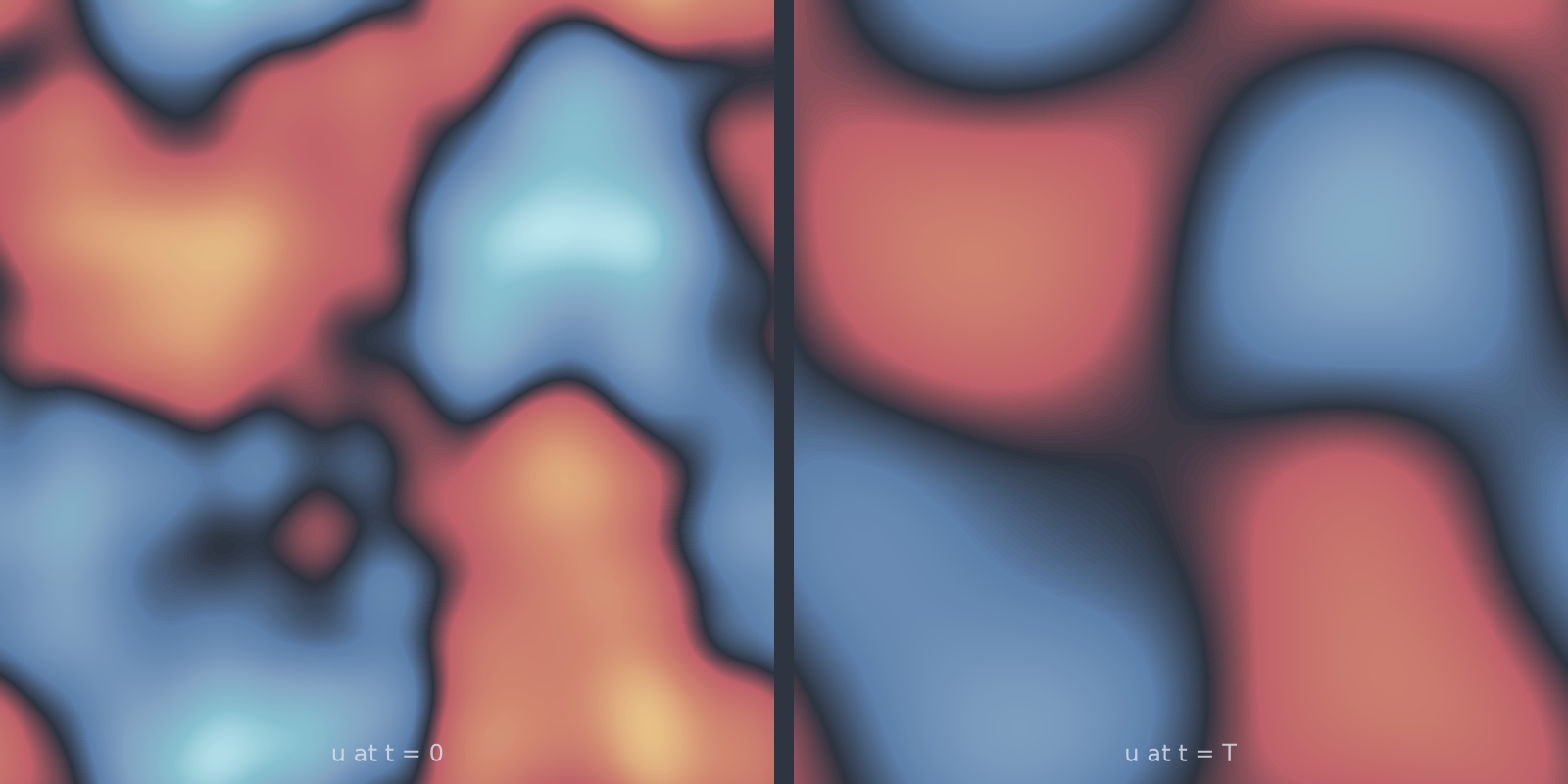
heat_2d): fine texture goes first, the large-scale pattern survives.Equation
with periodic boundary conditions.
Operator learning task
Parameters
| Parameter | Default | Range | Description |
|---|---|---|---|
diffusivity |
0.01 | (1e-6, 1.0) | Thermal diffusivity \(\alpha\) |
time_end |
1.0 | (0.01, 10.0) | Final time \(T\) |
Usage
from pdeforge import generate_dataset

dataset = generate_dataset(
    model="heat_2d",
    n_samples=1000,
    resolution={"x": 64, "y": 64},
    params={"diffusivity": 0.01, "time_end": 1.0},
    seed=42,
)
Solver
Exact spectral propagation, as in one dimension: fftn over both axes, the
symbol \(e^{-\alpha |\mathbf{k}|^2 t}\) applied once, one inverse transform. A
sample costs two FFTs regardless of the horizon.
Behaviour
The useful regime for a benchmark is the one where the output still carries structure the input does not trivially predict. Solving \(e^{-\alpha T |\mathbf{k}|^2} = 0.01\) at the default \(\alpha T = 0.01\) puts the 1%-of-amplitude cutoff at \(|\mathbf{k}| \approx 21\), which at \(64^2\) leaves most of the resolvable spectrum alive. Raising \(\alpha T\) to 0.1 drops that cutoff to \(|\mathbf{k}| \approx 7\), and the target starts to look like a handful of modes.
Data shapes
Related
heat_1d,heat_3d: the same model in one and three dimensions.stochastic_heat_2d: forced by space-time noise, with an ensemble per initial condition.allen_cahn_2d: diffusion plus a double-well reaction, which stops the smoothing and holds interfaces instead.