Helmholtz 2D (helmholtz_2d)
The frequency-domain scattering problem, with no time axis at all. The whole operator is one multiplier in Fourier space, \(1/(\kappa^2 - |\mathbf{k}|^2 + i\gamma\kappa)\), which makes it unusually legible: the response is nearly proportional to the source everywhere except near the resonant shell \(|\mathbf{k}| \approx \kappa\), where the denominator almost vanishes and the amplification is enormous. Where a dataset sits relative to that shell is the whole difficulty.
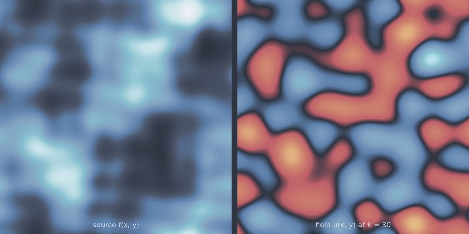
helmholtz_2d): a smooth, sub-resonant source, where the response reshapes the input rather than adding oscillation.Equation
on the periodic box. The small absorption term \(i\gamma\kappa\) models a lossy medium and, more practically, regularises the resonances: without it the periodic problem is singular whenever \(\kappa^2\) lands on an eigenvalue of the Laplacian. With it, every wavenumber is well posed.
Operator learning task
Parameters
| Parameter | Default | Range | Description |
|---|---|---|---|
wavenumber |
20.0 | (1.0, 200.0) | Helmholtz wavenumber \(\kappa\) |
damping |
1.0 | (0.001, 20.0) | Absorption \(\gamma\) |
Raising \(\kappa\) moves the resonant shell outwards, to \(|\mathbf{k}| = \kappa\). The default input measure is smooth and sits well inside that shell, so the default dataset is sub-resonant and comparatively easy. To reach the hard regime, excite the source near the shell: at \(\kappa = 20\) on the \(2\pi\) box that means an input measure carrying energy around wavenumber 20, and a grid several times finer again to resolve what comes back.
Lowering damping narrows the resonance and raises its peak, which makes the
operator stiffer to learn wherever the input measure touches the shell.
Usage
from pdeforge import generate_dataset

dataset = generate_dataset(
    model="helmholtz_2d",
    n_samples=1000,
    resolution={"x": 128, "y": 128},
    params={"wavenumber": 20.0, "damping": 1.0},
    seed=42,
)
Solver
Solved directly in Fourier space: the operator is diagonal there, so each mode is one complex division. The result is exact for the discrete operator to machine precision, and a sample costs two transforms. There is no iteration to converge and no time step to choose.
Behaviour
The interesting failure mode is spectral rather than spatial. A source with energy concentrated near \(|\mathbf{k}| = \kappa\) is amplified by the resonant denominator, so nearly all of the output's energy can come from a thin annulus in wavenumber space that the input barely populates. An operator that learns an averaged response across the spectrum will miss it, and no amount of spatial error analysis will show why.
The figure above is the opposite case, and worth reading as the baseline: a smooth source at \(\kappa = 30\) has almost no energy at \(|\mathbf{k}| = 30\), so the multiplier is close to the constant \(1/\kappa^2\) over the whole occupied band and the field is a reshaped version of the source rather than something new.
Data shapes
Related
wave_2d: the same physics in the time domain.heterogeneous_wave_2d: scattering off a varying medium rather than a varying source.darcy_2d: the other steady spectral solve.