Egg-shell droplets (`eggshell_droplets_3d`)

Two droplets coarsen inside the active shell of a catalyst pellet, and the model asks which of the two coarsening mechanisms carries them off. This is the classical dichotomy in supported-catalyst sintering, posed at the smallest system in which the two are separable:

Ostwald ripening. The droplets stay put and exchange material by diffusion through the matrix. The Gibbs-Thomson effect puts the chemical potential at a droplet of radius \(R\) at \(\sigma/R\), so the smaller partner sits at the higher potential, dissolves, and feeds the larger one.
Coalescence. The droplets touch, the interface between them bridges, and the pair merges with both partners still substantially intact.

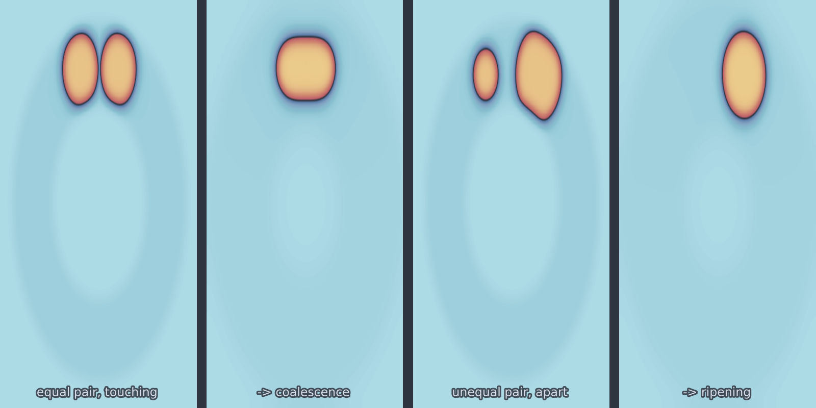
Egg-shell droplets — The two regimes, sliced through the plane containing both droplet centres. Left pair: equal droplets already touching merge with both partners intact. Right pair: unequal droplets held apart — the smaller one dissolves where it stands and never moves.

Both are already contained in the Cahn-Hilliard equation; neither has to be added. Exactly two droplets is the smallest configuration that separates them, and 3D is the dimension in which the question is well posed — the quasi-static diffusion field around a droplet falls off as \(1/r\) in three dimensions and so has a proper isolated limit, where in two dimensions it is logarithmic, no isolated droplet exists, and ripening rates depend on the size of the box.

Equation

\[\frac{\partial u}{\partial t} = \nabla\cdot\!\left(M(\mathbf{x})\,\nabla\mu\right), \qquad \mu = u^3 - u - \varepsilon^2\nabla^2 u\]

The geometry rides on the mobility rather than on the boundary conditions:

\[M(\mathbf{x}) = M_0\left[\phi_0 + (1-\phi_0)\,\psi(\mathbf{x})\right]\]

where \(\psi\) is a smoothed indicator of the spherical shell \(r_{\text{in}}(\hat{n}) \le |\mathbf{x}| \le r_{\text{out}}\) and \(\phi_0 \ll 1\) is the residual mobility of the inert support core. Where \(M\) is negligible there is no flux, so the core and the pellet exterior are frozen at \(u=-1\) and every bit of transport happens in the shell. That is what an egg-shell catalyst is: an impermeable core with the active phase confined to a thin outer layer.

Two consequences are worth stating plainly.

Mass is conserved exactly. The right-hand side is assembled in flux form, so the \(k=0\) Fourier mode of the update is identically zero and the drift is round-off — not a tolerance that has to be tuned, and not something the geometry or the noise can spoil.

The shell is integrated by the standard stepper. For constant \(M\) the flux form telescopes to \(-M k^2 \hat{\mu}\) and the stabilised IMEX step becomes the cahn_hilliard update exactly, numerator and denominator alike. Since \(M = M_0\) throughout the active shell, the variable coefficient is only ever felt where nothing is happening.

The shell is also a closed domain, so unlike a periodic box there are no periodic-image artefacts in the diffusion field: the two droplets see each other around the sphere both ways, and the reservoir available to them is finite and known.

Operator learning task

\[\left(u(\mathbf{x},0),\; M(\mathbf{x})\right) \mapsto u(\mathbf{x},T)\]

The shell geometry travels with the sample as a second input channel. With shell_roughness on it differs from sample to sample, and a surrogate cannot predict the dynamics without it.

The outcome bifurcates: a small change in the initial configuration flips the pair between macroscopically different end states. That makes the map a deliberately hard one to learn and a sharp test of whether a surrogate's uncertainty is honest near the boundary.

Parameters

Parameter	Default	Range	Description
`epsilon`	0.010	(0.006, 0.03)	Interface width; \(\sigma = 2\sqrt{2}\varepsilon/3\)
`mobility`	1.0	(0.01, 10.0)	Mobility \(M_0\) in the active shell
`shell_outer`	0.44	(0.15, 0.48)	Outer pellet radius, box units
`shell_thickness`	0.20	(0.02, 1.0)	Active layer thickness — the confinement knob
`shell_roughness`	0.0	(0.0, 0.6)	Relative amplitude of random thickness variation
`shell_corrugation`	0.0	(0.0, 0.8)	Egg-carton corrugation amplitude
`corrugation_modes`	6.0	(2.0, 14.0)	Bumps around a great circle
`droplet_radius`	0.09	(0.02, 0.14)	Mean droplet radius \(\bar{R}\)
`size_asymmetry`	0.15	(0.0, 0.5)	\((R_1-R_2)/(R_1+R_2)\) — the ripening drive
`droplet_gap`	1.0	(0.05, 6.0)	Surface-to-surface gap in units of \(\bar{R}\)
`noise_intensity`	0.0	(0.0, 1e-5)	Conserved thermal noise \(\Theta\)
`time_end`	0.3	(0.001, 5.0)	Final time

Which knob selects the regime

droplet_gap decides the outcome, and it decides it almost alone. A sweep of gap against asymmetry at \(128^3\), 37 runs:

asym \ gap	0.15	0.25	0.28	0.31	0.34	0.37	0.40	0.60	0.90	1.40	2.00
0.00	coal	coal	coal	coal	coal	coal	coal	—	—	—	—
0.16	coal	coal	coal	coal	coal	coal	coal	ripe	ripe	ripe	ripe
0.35	coal	coal	coal	coal	coal	ripe	ripe	ripe	ripe	ripe	ripe

The reason the gap dominates is a separation of timescales, and it is worth being explicit about because it is easy to expect otherwise. Bridging is an interface-relaxation process: once the diffuse interfaces overlap it completes in a time set by \(\varepsilon\) and the mobility, far faster than anything diffusive. Ripening is diffusive, taking \(t \sim 2R^3/(M\sigma)\). So wherever bridging is possible at all it wins outright, and wherever it is not, ripening is the only channel left.

size_asymmetry moves the boundary, but only near it. It controls the driving force \(\sigma(1/R_2 - 1/R_1)\), hence how fast the ripening branch runs and how far the survival fraction falls. Raising it from 0.16 to 0.35 pulls the boundary in from between \(0.40\) and \(0.45\,\bar{R}\) to between \(0.34\) and \(0.37\) — a real but confined effect, exactly where the two timescales become comparable. The size of that shift is not free: equating the two rates gives \(g^*(a) = \text{const} - (\varepsilon/\sqrt2)\ln a\), predicting \(0.0055\), against \(0.0063\) measured.

The dashes on the top row are not gaps in the sweep. At zero asymmetry there is no ripening drive at all, so a well-separated pair simply persists: those runs reach time_end with both droplets intact and are reported unresolved, which is the honest answer there. See the warning below.

shell_thickness holds the pair apart as it tightens. Measured at gap \(0.31\), asymmetry \(0.16\), the contact gap at the event widens monotonically as the shell closes in, while the survival fraction stays high:

shell thickness	0.10	0.14	0.20	0.28
contact gap (\(\varepsilon\))	4.87	3.57	2.87	2.77
\(\rho\)	0.913	0.929	0.947	0.947
regime	`mixed`	`coal`	`coal`	`coal`

Squeezing the droplets into lenses spreads them laterally within the layer and keeps their cores further apart, so the pair that merges comfortably in a roomy shell is, at \(\delta = 0.10\), already on the boundary. Confinement therefore acts against coalescence rather than for it — the same direction the egg-carton corrugation pushes, and for the same reason.

Zero asymmetry is an unstable equilibrium

At size_asymmetry = 0 the partners are identical, so there is no Gibbs-Thomson difference and nothing selects which of them dissolves. The pair sits on a knife edge, and in a deterministic run the tie is broken by the grid — the two centres fall at different sub-cell offsets — which is an artefact, not physics. In the sweep those runs simply persist to time_end and are reported unresolved, which is the correct answer for a pair with no reason to change. This is precisely what noise_intensity is for: with conserved thermal noise the symmetry is broken physically and the outcome becomes a distribution over seeds rather than a single answer. Away from the line, the asymmetry dominates any grid effect and deterministic runs are meaningful on their own.

The matrix does not start at \(u=-1\)

A droplet of radius \(R\) is only in local equilibrium with a matrix at \(-1 + \sigma/(2R)\). Against a matrix at exactly \(-1\) both droplets simply evaporate, and since the shell reservoir is far larger than the droplets they evaporate completely. The shell matrix is therefore seeded at the Gibbs-Thomson supersaturation for the mean radius, which puts the critical radius at \(\bar{R}\) and makes this an exchange problem — larger droplet grows, smaller dissolves — rather than a dissolution problem.

Crucially the supersaturation is applied uniformly, not just inside the shell. Seeding the active layer at \(-1+\delta u_0\) while leaving the inert core and exterior at \(-1\) would put a chemical potential step across the shell wall, and the frozen region is around 60% of the box — an enormous sink whose mobility is small but not zero. It drains the active layer steadily: with the step in place a symmetric pair lost 20% of its volume by \(t=0.03\) and the survivor of a ripening pair shrank, masking the very mechanism the model exists to show. Levelling the potential removes the driving force, cutting the loss to about 6% and restoring the proper Ostwald signature — the larger droplet growing as the smaller dissolves. What the frozen region holds is arbitrary anyway, since nothing flows there once there is no gradient to drive it.

The remaining few per cent is the genuine residue: \(\delta u_0\) is the linearised Gibbs-Thomson value taken about \(u=-1\), and confined droplets are lenses rather than spheres, so it is close to the true equilibrium but not equal to it. Total droplet volume is therefore not itself conserved — only \(\int u\) is, and that to machine precision.

Resolution follows epsilon

The interface needs about four points across it, so \(\varepsilon \gtrsim 1.3\,\Delta x\), and quantitative Gibbs-Thomson wants \(R/\varepsilon \gtrsim 8\). The defaults are tuned for \(128^3\).

Regime classification

Every run is classified automatically. Connected components of \(\{u>0\}\) are tracked frame by frame and the pair is labelled at the moment the count drops from two to one, using two independent signals.

Were they ever in contact? The surface-to-surface gap at the last frame where both droplets exist, in units of \(\varepsilon\), with each radius taken from its measured volume as \((3V/4\pi)^{1/3}\). Merging requires contact by definition and dissolving at a distance forbids it, so the question separates the mechanisms exactly. It is also the only signal that survives coarse output sampling — a dissolving droplet's last moments are abrupt, so its final recorded volume is frame-dependent, but its distance from its neighbour is not. Measured populations are far apart: pairs that merged register \(0.6\)–\(1.5\,\varepsilon\), pairs that ripened \(6.6\,\varepsilon\) and up.

Asking where the material went does not work

It is tempting to separate the mechanisms by asking whether the survivor absorbed its partner. It does not discriminate: in Ostwald ripening the surviving droplet ends up with the material too — that is precisely what ripening is. The difference is that it arrives gradually, by diffusion through the matrix, rather than all at once. The absorbed fraction is reported because it is informative, but it decides nothing.

How much was left to take part? The survival fraction

\[\rho = \frac{V_{\text{small}}(t_{\text{event}})}{V_{\text{small}}(0)}\]

then grades the merger, separating a genuine merger of two healthy droplets from an already-dissolving remnant being mopped up. It is a continuous regime coordinate, not just a label:

contact gap	\(\rho\)	Regime
\(\le 3\,\varepsilon\)	\(\ge 0.5\)	`coalescence`
\(\le 3\,\varepsilon\)	\(< 0.5\)	`mixed` — touched, but only after substantial ripening
\(> 3\,\varepsilon\)	any	`ripening` — they never met
—	pair still intact at \(T\)	`unresolved`

The threshold is physical rather than fitted: diffuse interfaces interact once they are within about one interface thickness, \(2\sqrt{2}\varepsilon = 2.83\,\varepsilon\).

Centroid approach is reported as a third, weaker signal: coalescing droplets migrate together, ripening ones stay put.

Diagnostics from the last solve — per-frame volumes, component counts, centroid separations, and the labels above — are left on model.last_diagnostics.

Usage

from pdeforge import get_model

model = get_model("eggshell_droplets_3d")(
    resolution={"x": 128, "y": 128, "z": 128},
    size_asymmetry=0.25,
    droplet_gap=1.0,
)
ic = model.generate_ic(seed=0)      # (2, 128, 128, 128): u0 and M
u_T = model.solve(ic)
print(model.last_diagnostics["regime"])       # -> 'ripening'

Selecting the other regime is a matter of removing the ripening drive and letting the interfaces touch:

model = get_model("eggshell_droplets_3d")(
    resolution={"x": 128, "y": 128, "z": 128},
    size_asymmetry=0.0,     # no Gibbs-Thomson difference between partners
    droplet_gap=0.15,       # interfaces already overlapping
    time_end=0.05,
)
ic = model.generate_ic(seed=0)
model.solve(ic)
print(model.last_diagnostics["regime"])       # -> 'coalescence'

The two mechanisms, side by side

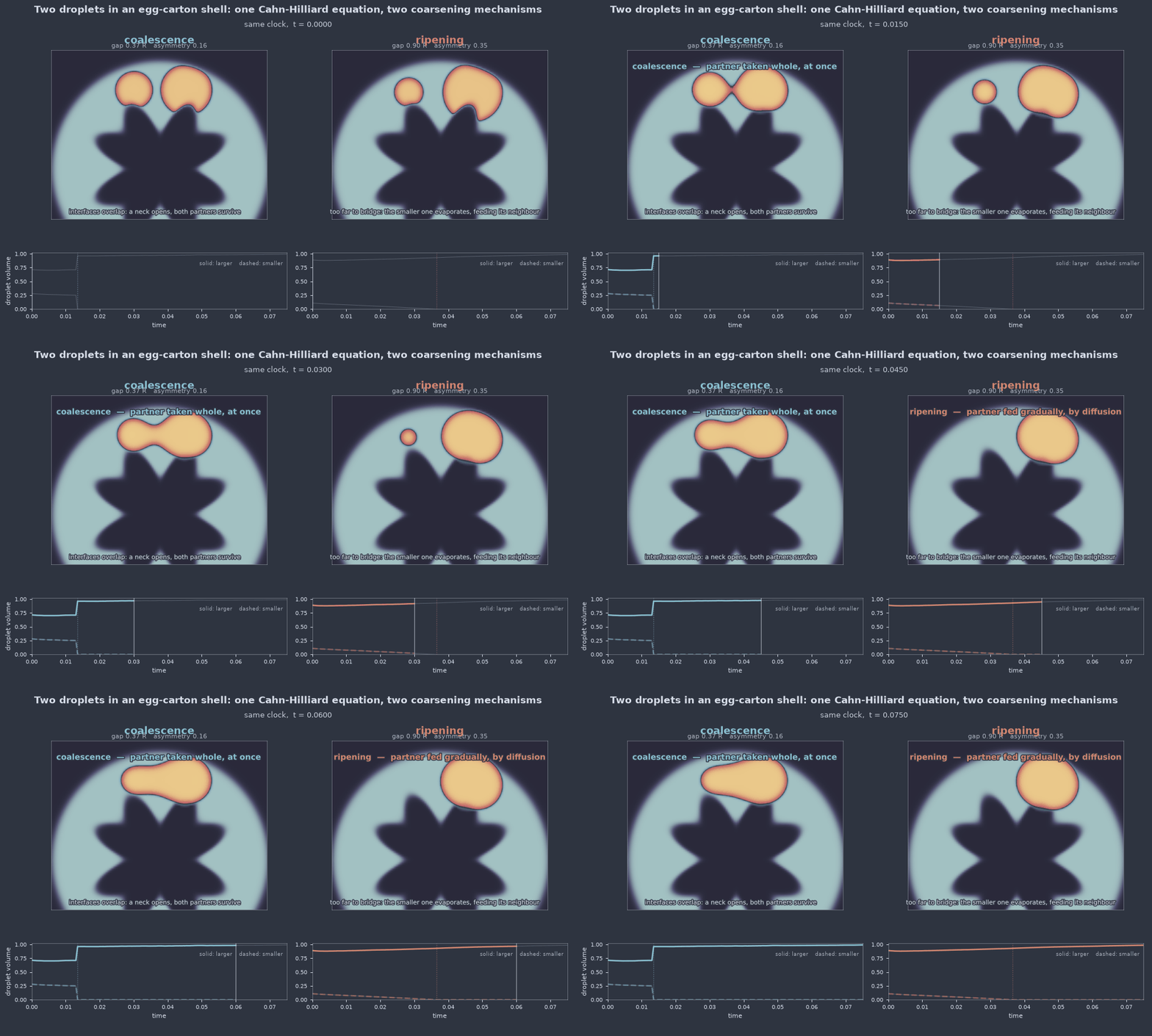
Coarsening animation — Both mechanisms on one shared clock, sliced through the plane containing both droplet centres. The pale annulus is the active shell and the dark lobed core is the egg-carton corrugation cut through the mid-plane. The tell is in the volume traces: coalescence takes its partner in a single jump, ripening receives it gradually, by diffusion.

The pair shown is chosen so both events fall at nearly the same physical time, so what differs on screen is the mechanism rather than the pacing.

Measured behaviour

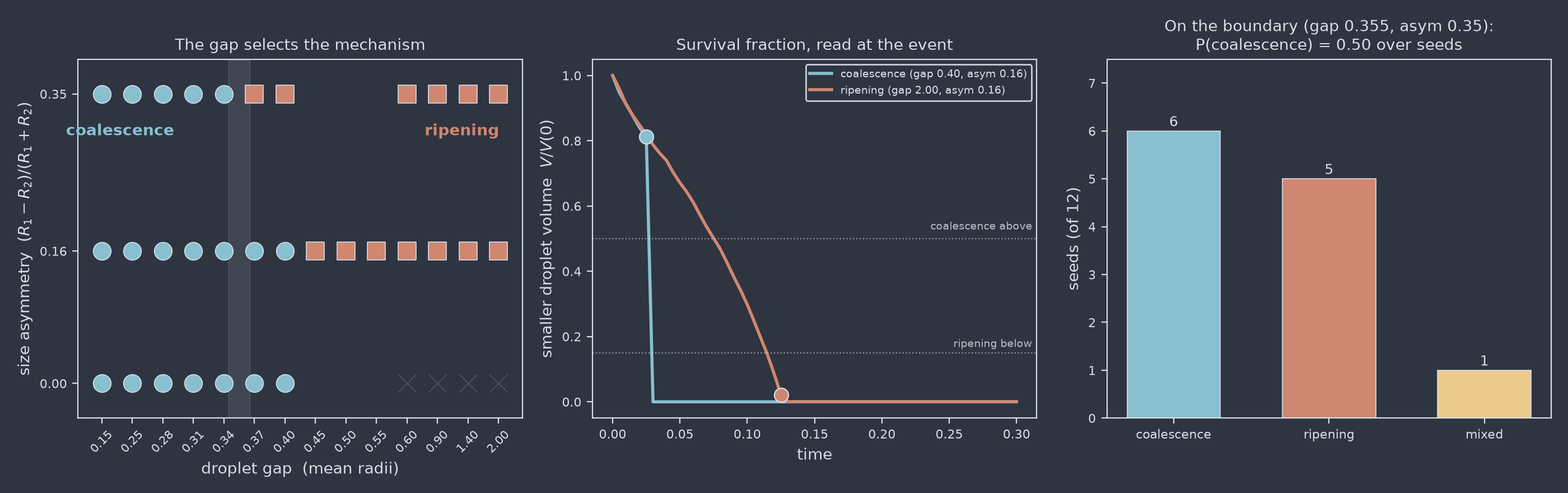
Phase diagram — Left: the regime as a function of gap and asymmetry at 128³, with the boundary band shaded. Centre: the smaller droplet's volume through a run of each kind, with the survival fraction read at the marked event. Right: on the zero-asymmetry line, where the deterministic problem is a knife edge, conserved noise turns the outcome into a distribution over seeds: on the boundary itself the split is 6 coalescence to 5 ripening, while the deterministic run cannot decide at all.

The boundary is sharp, lives in the gap, and is not vertical. Resolving the window between \(0.28\) and \(0.60\) shows it tilting with asymmetry, exactly where the two timescales become comparable:

gap	asym 0.00	asym 0.16	asym 0.35
0.31	coal (\(\rho\) 0.977)	coal (0.947)	coal (0.848)
0.34	coal (0.976)	coal (0.942)	coal (0.719)
0.37	coal (0.970)	coal (0.910)	ripe (0.139)
0.40	coal (0.959)	coal (0.812)	ripe (0.137)
0.60	—	ripe (0.034)	ripe (0.013)

Inside the coalescence region the survival fraction falls steadily with asymmetry at fixed gap, so the continuous coordinate registers the competition long before the label does.

The two populations are widely separated in both signals, which is what makes the classification robust rather than a matter of where a threshold sits:

	contact gap	\(\rho\)
merged	1.31 – 3.77 \(\varepsilon\)	0.719 – 1.000
ripened	5.71 – 9.71 \(\varepsilon\)	0.013 – 0.139

Across all 37 runs the two never disagreed, and no run was labelled mixed.

Mass drift over the whole sweep peaked at \(4.4\times10^{-16}\).

Validation

The model carries the invariants that pin it down:

mass conserved to machine precision, with and without noise and roughness;
free energy monotonically decreasing, since \(dF/dt = -\int M|\nabla\mu|^2 \le 0\) for any non-negative mobility;
the constant-mobility step reproducing the cahn_hilliard update to \(4\times10^{-16}\);
the smaller droplet being the one that dissolves, as Gibbs-Thomson requires;
both regimes reachable, and selected by the documented knobs.

Egg-shell droplets (eggshell_droplets_3d)