Rayleigh-Bénard 2D (rayleigh_benard_2d)
Buoyancy-driven convection in a closed cavity, and the model with a genuine bifurcation in it. Below the critical Rayleigh number the fluid does not move at all and heat crosses by conduction; above it, convection rolls set in. Which roll state the flow settles into depends on the initial perturbation, so a Rayleigh sweep with per-sample perturbations gives parametric and structural variability at once.
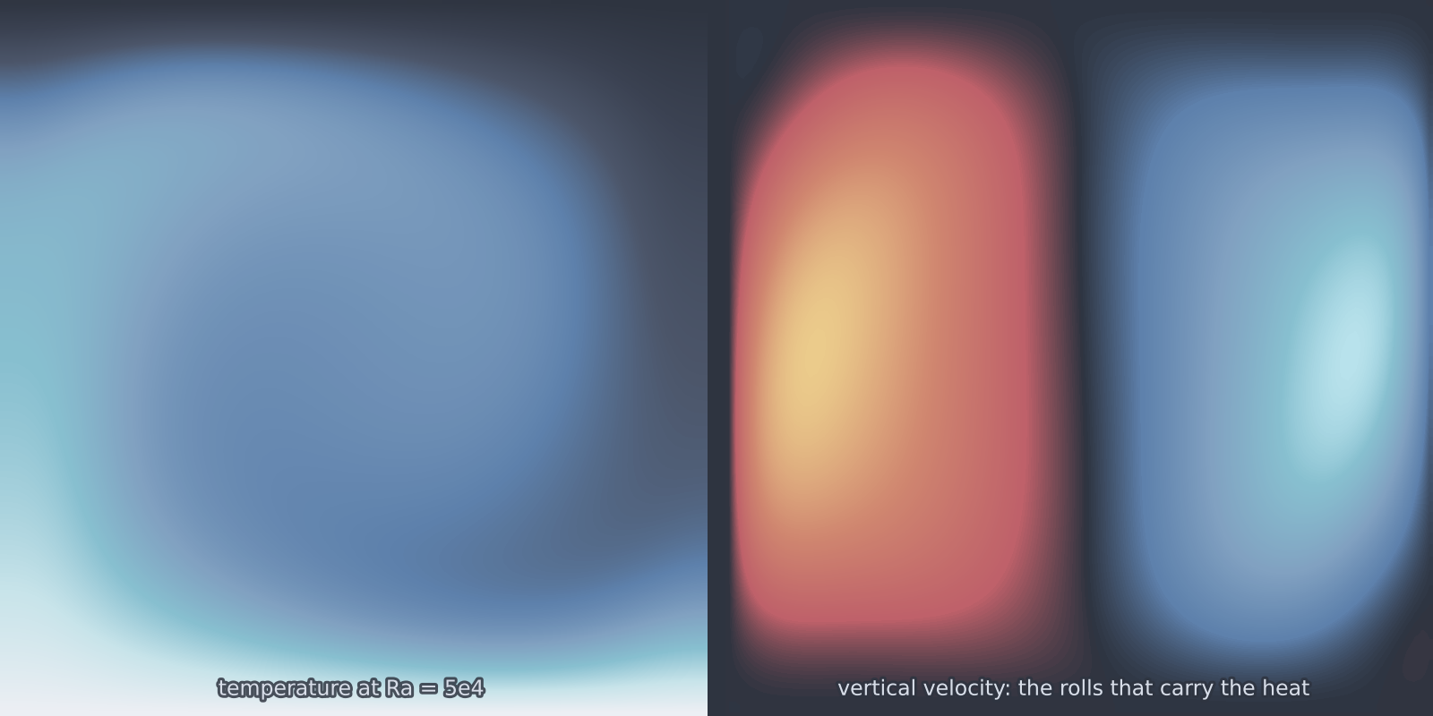
rayleigh_benard_2d): convection rolls carry heat from the hot plate to the cold one.Equations
Boussinesq, nondimensionalised on the cavity height and the thermal diffusion time:
No-slip on all walls, \(T = 1\) on the bottom plate, \(T = 0\) on the top, and adiabatic sidewalls.
Operator learning task
Parameters
| Parameter | Default | Range | Description |
|---|---|---|---|
rayleigh |
1e4 | (100, 1e6) | Rayleigh number; onset at \(\mathrm{Ra}_c \approx 1708\) |
prandtl |
0.71 | (0.01, 100.0) | Prandtl number |
time_end |
0.5 | (0.01, 10.0) | March time in thermal-diffusion units |
perturbation |
0.05 | (0.0, 0.5) | Amplitude of the random initial temperature perturbation |
Below \(\mathrm{Ra}_c \approx 1708\) the conduction state \(T = 1 - y\) is stable and the Nusselt number is exactly 1. Above it, rolls set in and Nusselt grows.
Usage
from pdeforge import generate_dataset

dataset = generate_dataset(
    model="rayleigh_benard_2d",
    n_samples=20,
    resolution={"x": 64, "y": 64},
    params={"rayleigh": 1e4, "prandtl": 0.71},
    seed=42,
)
The plate-averaged Nusselt numbers are computed on every solve and returned in that sample's validation record, alongside the top-to-bottom flux imbalance that the record is checked against.
This model needs FEniCSx. See FEniCSx setup.
Solver
Semi-implicit Oseen steps, with advection linearised at the previous velocity and diffusion implicit, on Taylor-Hood P2/P1 elements with one pressure degree of freedom pinned, followed by an implicit advection-diffusion step for the temperature on P2.
Validation
The Nusselt number is the plate-averaged \(-\partial T/\partial y\). At steady state the bottom and top values must agree, and the sub-critical cavity must return exactly 1. Measured in July 2026: at \(\mathrm{Ra} = 10^4\), \(\mathrm{Pr} = 0.71\) on a 48x48 Taylor-Hood mesh the model gives \(\mathrm{Nu} = 2.155\) at the bottom and \(2.162\) at the top, a 0.3% flux imbalance, against the square-cavity benchmark value 2.158 of Ouertatani et al. (2008). At \(\mathrm{Ra} = 800\) the cavity returns \(\mathrm{Nu} = 1.000\) with the velocity decaying to zero.
Behaviour
Roll multiplicity is what makes this model interesting and awkward at the same time. Several steady roll states coexist at the same Rayleigh number, and the initial perturbation selects between them, so two samples with identical parameters can converge to different flows. That is physics rather than solver noise, and an operator that maps parameters to a single field cannot represent it. Treat the perturbation as part of the input, or expect an irreducible error floor.
Data shapes
dataset.inputs.shape   # (n_samples, nx, ny)      the initial T perturbation
dataset.outputs.shape  # (n_samples, nx, ny, 3)   u, v, T
The FEniCSx models store space as (nx, ny) with the component axis trailing,
transposed relative to the spectral models' (ny, nx).
Related
cylinder_flow_2d_unsteady: the other FEniCSx model with a bifurcation, in that case to vortex shedding.shallow_water_2d: buoyancy-free flow on a periodic box.