Schrödinger 1D (schrodinger_1d)

The nonlinear Schrödinger equation, and the only complex-valued model in the catalogue. Two properties make it worth having: the dynamics are dispersive rather than dissipative, so nothing is smoothed away, and the solver conserves the \(L^2\) norm to machine precision, which gives every generated sample a scalar invariant you can check without a reference solution.

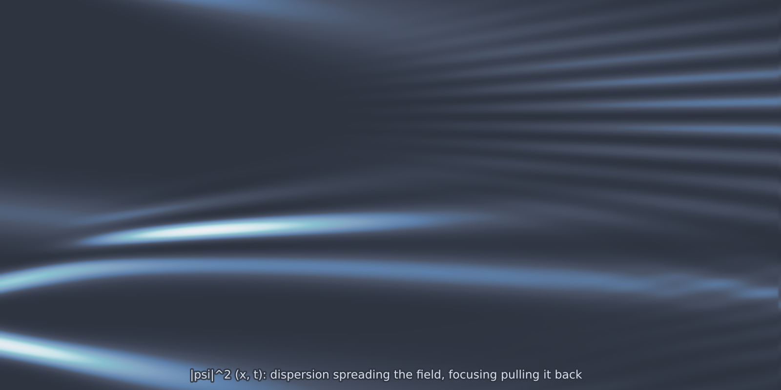
Space-time density |psi|² (schrodinger_1d): dispersion spreads the field while the focusing nonlinearity pulls it back into bright filaments.

Equation

\[i\,\frac{\partial \psi}{\partial t} = -\tfrac{1}{2}\,\frac{\partial^2 \psi}{\partial x^2} + g\,|\psi|^2\,\psi\]

on a periodic domain. Negative \(g\) is the focusing case, where bright solitons exist; positive \(g\) defocuses.

Operator learning task

\[\big(\operatorname{Re}\psi, \operatorname{Im}\psi\big)(x, 0) \;\mapsto\; \big(\operatorname{Re}\psi, \operatorname{Im}\psi\big)(x, T)\]

The complex field is exposed as two real channels of shape (2, nx), so standard real-valued architectures need no special handling.

Parameters

Parameter	Default	Range	Description
g	-1.0	(-10.0, 10.0)	Nonlinearity; \(g < 0\) focusing, \(g > 0\) defocusing
time_end	1.0	(0.01, 50.0)	Final time \(T\)

Usage

from pdeforge import generate_dataset

dataset = generate_dataset(
    model="schrodinger_1d",
    n_samples=1000,
    resolution={"x": 256},
    params={"g": -1.0, "time_end": 1.0},
    seed=42,
)

Solver

Strang split-step Fourier. The dispersive half-step is exact in Fourier space and the nonlinear phase rotation is exact pointwise, so each piece of the splitting is solved without error and only their non-commutation contributes, at \(O(\Delta t^2)\). Total power \(\int |\psi|^2\,dx\) is conserved to machine precision, which is the model's built-in validation invariant.

Behaviour

The focusing branch is the one that produces structure. At \(g < 0\) an initially broad field can self-concentrate into narrow, tall peaks, and because there is no dissipation those peaks persist and recur rather than relaxing. The defocusing branch spreads instead, and gives a considerably easier target.

Data shapes

dataset.inputs.shape   # (n_samples, 2, nx)   Re psi, Im psi at t = 0
dataset.outputs.shape  # (n_samples, 2, nx)   the same at t = T

Related

• kdv_1d: the other dispersive 1D model, with solitons that survive collision.
• wave_1d: non-dispersive propagation for comparison.