Kolmogorov flow 2D (kolmogorov_flow_2d)
Forced two-dimensional turbulence. A steady sinusoidal band force injects energy at a single wavenumber, the nonlinearity cascades it across scales and viscosity dissipates it, and at low viscosity the result is a statistically steady turbulent state rather than a decaying one. That steadiness is what makes this the right model for long-horizon work: the statistics of the target do not drift with \(T\), so a horizon can be lengthened without also changing what is being asked.
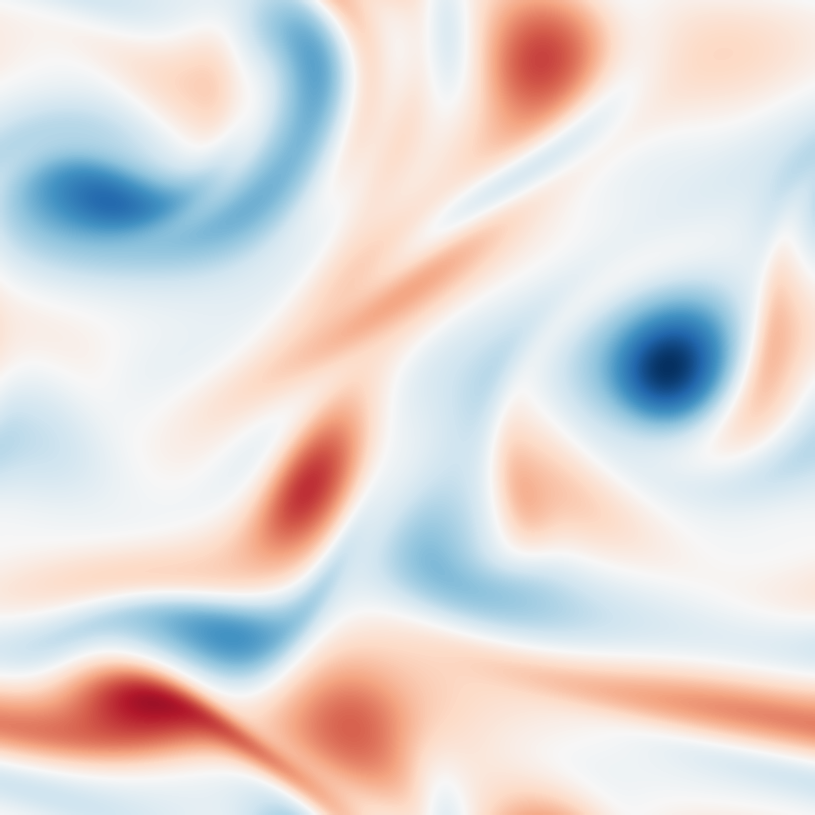
kolmogorov_flow_2d): viscosity sets the Reynolds number.Equation
The Navier-Stokes vorticity dynamics of ns_vorticity_2d
driven by \(\mathbf{f} = (f_0 \sin(n y),\, 0)\), which in vorticity form
contributes
on the \(2\pi\)-periodic box.
Operator learning task
Parameters
| Parameter | Default | Range | Description |
|---|---|---|---|
viscosity |
0.025 | (1e-4, 1.0) | Kinematic viscosity, \(1/\mathrm{Re}\); lower is more turbulent |
forcing_wavenumber |
4 | (1, 16) | Band-forcing wavenumber \(n\) |
forcing_amplitude |
1.0 | (0.0, 10.0) | Forcing amplitude \(f_0\) |
time_horizon |
10.0 | (0.1, 200.0) | Final time \(T\) |
forcing_wavenumber sets how many bands the forcing lays across the box, and
so the scale at which energy enters. It is visible in the output: the figure
above is \(n = 4\).
Usage
from pdeforge import generate_dataset

dataset = generate_dataset(
    model="kolmogorov_flow_2d",
    n_samples=500,
    resolution={"x": 128, "y": 128},
    params={"viscosity": 1/70, "forcing_wavenumber": 4, "time_horizon": 30.0},
    backend="jax",
    seed=7,
)
The JAX backend is worth using here: the horizons that reach a developed turbulent state are long, and the solver is a good fit for accelerator execution.
Solver
Inherited from ns_vorticity_2d: ETDRK4 with exact
viscous diffusion and dealiased explicit advection, plus the steady forcing
term added to the right-hand side.
Behaviour
At \(\nu = 0.025\) the flow is smooth and the band structure of the forcing remains visible in the solution. Around \(\nu = 1/70\) the cascade takes over and the field develops the filamentary vorticity texture of two-dimensional turbulence. Below roughly \(\nu = 10^{-3}\) at \(128^2\) the finest structures reach the grid scale, and the dataset begins to record the discretisation.
Data shapes
Related
ns_vorticity_2d: the unforced parent model and the published benchmark family.ks_1d: chaos in one dimension, where the attractor is small enough to characterise.cylinder_flow_2d_turbulent: wall-bounded turbulence under a large-eddy closure.