Heterogeneous Wave 2D (heterogeneous_wave_2d)
Waves through a random medium, and the one model in the catalogue whose operator task is shaped like an inverse problem. The source pulse is fixed and identical for every sample; what varies is the medium itself. Learning the map therefore means learning how a speed field bends, focuses and delays a wavefront, which is the forward operator that travel-time tomography inverts.
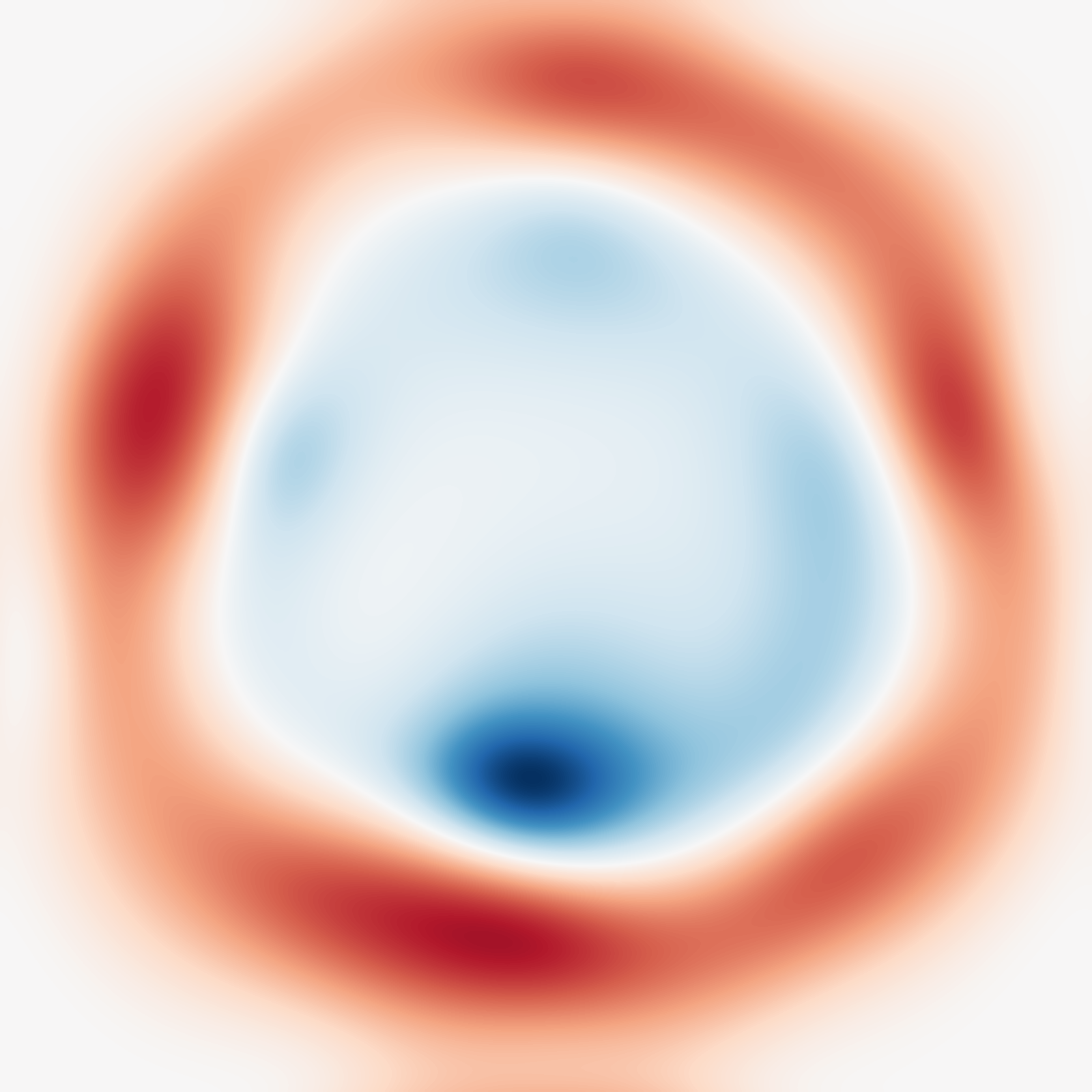
heterogeneous_wave_2d): c_min and c_max set the medium's contrast.Equation
on the periodic box, started from a fixed seeded Gaussian pulse.
Operator learning task
The input is the medium, and the output is the wavefield at the horizon. Because the source never changes, every difference between two samples is attributable to the medium.
Parameters
| Parameter | Default | Range | Description |
|---|---|---|---|
c_min |
0.5 | (0.05, 10.0) | Minimum wave speed |
c_max |
1.5 | (0.1, 20.0) | Maximum wave speed |
time_end |
0.3 | (0.01, 10.0) | Propagation time \(T\) |
pulse_width |
0.05 | (0.005, 0.5) | Width of the fixed source pulse |
The contrast \(c_{\max}/c_{\min}\) governs how strongly the medium refracts. At
the default 3, wavefronts visibly bend and focus; near 1 the model degenerates
into wave_2d with a constant speed.
Usage
from pdeforge import generate_dataset

dataset = generate_dataset(
    model="heterogeneous_wave_2d",
    n_samples=1000,
    resolution={"x": 128, "y": 128},
    params={"c_min": 0.5, "c_max": 1.5, "time_end": 0.3},
    seed=42,
)
Solver
Pseudo-spectral Laplacian with Störmer-Verlet (leapfrog) time-stepping. For
constant \(c\) the scheme's dispersion matches the exact spectral propagator to
\(O(\Delta t^2)\), and that agreement against wave_2d is the
model's validation invariant.
Behaviour
Longer horizons let the pulse interact with more of the medium, so more of the input field influences the output and the task gets harder in an interpretable way. Short horizons leave most of the domain untouched by the wave, which means most of the input carries no signal at all: a useful property if you want a task where the operator must learn where to look.
Data shapes
dataset.inputs.shape   # (n_samples, ny, nx)   the speed field c
dataset.outputs.shape  # (n_samples, ny, nx)   the wavefield at T
Related
wave_2d: the constant-speed case, and the validation reference.helmholtz_2d: scattering posed in the frequency domain.darcy_2d: the other coefficient-to-field map in the catalogue.