Heat 1D (heat_1d)
Diffusion is the one operator whose behaviour you can predict before you run
anything: every Fourier mode decays at its own rate \(e^{-\alpha k^2 T}\), so
high wavenumbers vanish first and the solution map is a low-pass filter with a
known cutoff. That makes heat_1d the baseline every other time-dependent
model in the catalogue is read against. If a network cannot learn this map, the
problem is the network.
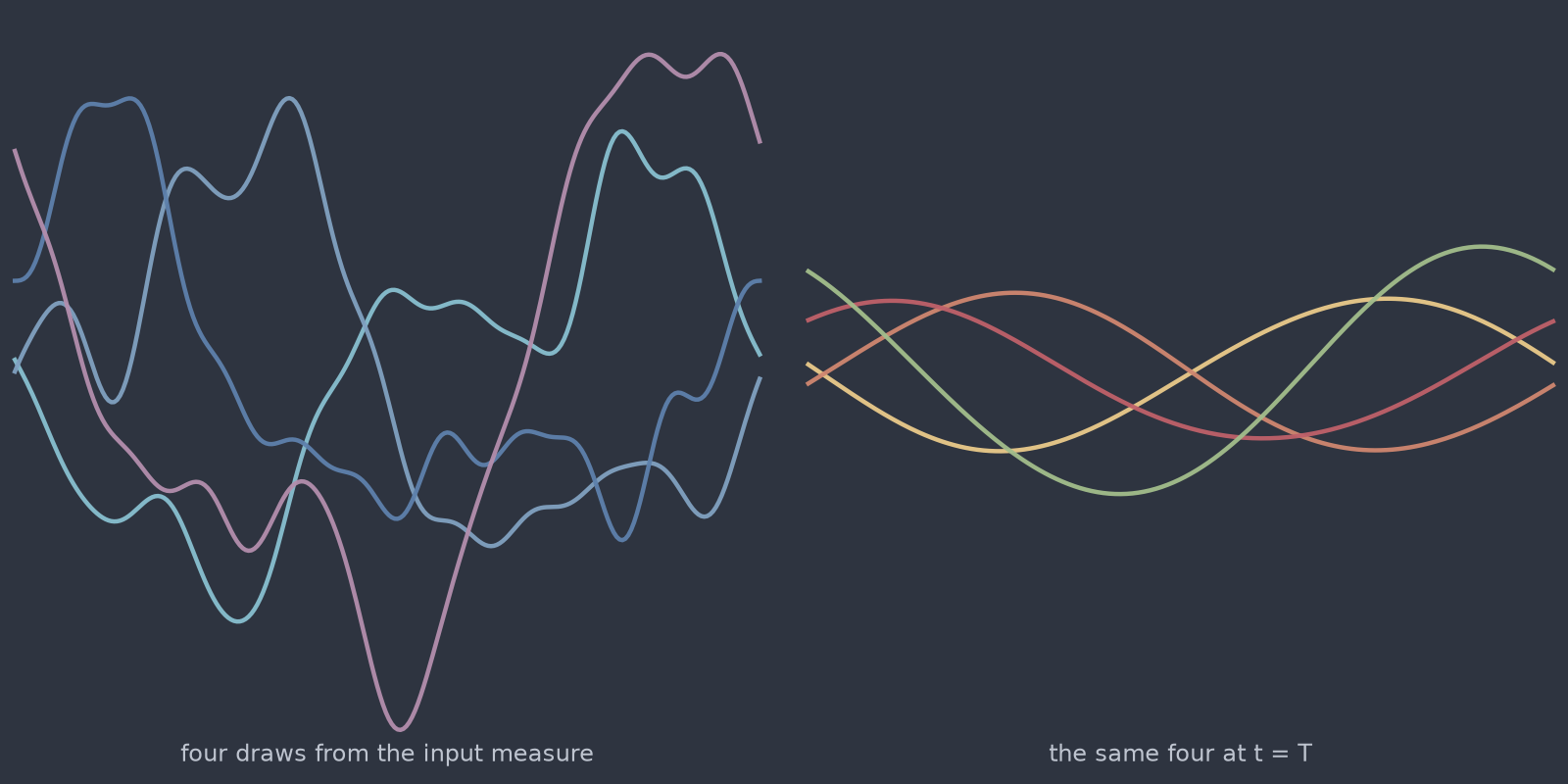
heat_1d): the operator strips high wavenumbers and leaves the slowest modes standing.Equation
with periodic boundary conditions on \([0, 2\pi]\).
Operator learning task
Parameters
| Parameter | Default | Range | Description |
|---|---|---|---|
diffusivity |
0.01 | (1e-6, 1.0) | Thermal diffusivity \(\alpha\) |
time_end |
1.0 | (0.01, 10.0) | Final time \(T\) |
Only the product \(\alpha T\) matters: doubling the diffusivity and halving the horizon gives the same operator. Pick whichever of the two reads better in the experiment you are describing.
Usage
from pdeforge import generate_dataset

dataset = generate_dataset(
    model="heat_1d",
    n_samples=1000,
    resolution={"x": 256},
    params={"diffusivity": 0.01, "time_end": 1.0},
    seed=42,
)
Solver
The linear symbol \(-\alpha k^2\) is applied exactly in Fourier space, so there
is no time-stepping error at all: the discrete solution is the exact solution
of the discrete problem, to machine precision. time_end therefore costs
nothing, and a horizon of 10 is as cheap as a horizon of 0.01.
Behaviour
At \(\alpha T \gtrsim 0.1\) on the \(2\pi\) box, everything above \(k \approx 3\) has decayed by more than a factor of \(e\), and the target fields become close to low-order trigonometric polynomials. Datasets generated there are easy to the point of being uninformative: an operator can score well by learning to output the first few modes. For a benchmark with something left to resolve, keep \(\alpha T\) near 0.01.
Data shapes
Related
heat_2dandheat_3d: the same solver on the square and the cube.stochastic_heat_1d: the same equation driven by space-time noise, which is where the uncertainty work starts.advection_1d: the other exactly-propagated linear model, and the one that tests phase rather than amplitude.